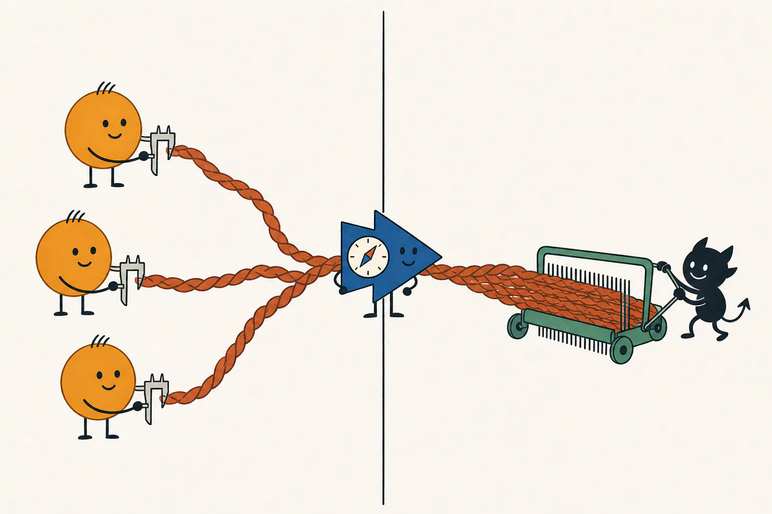
The Core Story showed good predictors fitting badly. One training example reveals why; adding examples explains the two sample thresholds.
If you landed here first:benign misfitting means predicting fresh examples well while fitting the training examples worse than predicting zero. Here, orthogonal nuisance directions let us derive what fitting costs.
Gireeja Ranade · Anant Sahai — UC Berkeley · companion to the stylized preprint
Simplify the example, keep the mechanism
One training point is enough to explain the mismatch.
Keep the signal coordinate that determines the label and the nuisance coordinates it ignores. A predictor in this one-example training span has one knob: how much of that example to use.
Freeze the training target at y = 1 and write its input as x_train = (√γ, z), in d input dimensions, with nuisance energy ‖z‖² = (d−1), equal to the number of nuisance coordinates. In fresh data, the signal coordinate has variance γ. The Core Story calls γ spike strength, or feature quality.
A fresh example is still Gaussian: x = (√γ s, z_fresh), y = s. Here s and the entries of z_fresh are independent standard Gaussians. Its nuisance has no reason to line up with the training point's.
Every predictor in this one-point span is u = α x_train. Its prediction is the inner product ⟨u, x⟩. Increasing α strengthens both the useful signal and the nuisance it carries.
one training example x_train
√γshared signal
z₁z₂…z₍d−1₎its own nuisance direction
↓
targety = 1
We score mean squared error: t over the training examples (one point here), g in expectation on fresh points. Predicting zero scores 1 on both in this cartoon. The early cartoons use separate examples; the later Gaussian-ray comparison returns to the Core Story’s opening draw.
Why interpolation stops too soon
Fitting gives nuisance credit for doing the signal's job.
On the training point, the predictor’s nuisance is a scaled copy of the point’s own nuisance, so the two line up perfectly. The prediction has two parts:
αγ + α(d−1)
In the full feature space, one clean label leaves infinitely many predictors that fit it: underspecification. The shortest of them, the minimum-norm interpolator, has α = 1/(γ + d−1), so the signal supplies only γ/(γ + d−1) of the training prediction. At the starting settings, γ = 30, d−1 = 199: 13% comes from signal, 87% from its own nuisance.
A fit that used the signal direction alone would have norm 1/√γ, about 0.183 here. The shortest fit has norm 1/√(γ+d−1), about 0.066. Using the point’s own nuisance makes fitting almost three times cheaper in norm. The signal-only fit would also need to know the hidden signal direction; Why the Span? shows what the observations leave unresolved.
A fresh point cannot count on that help. Its nuisance contribution has mean zero and variance (d−1)α², giving fresh-test error
g(α) = (1 − αγ)² + (d−1)α²
Moving beyond interpolation restores the missing signal. The best in span balances the signal still missing against nuisance variance; calibration goes farther and restores the signal completely. Meanwhile, the training point gets its own nuisance back on top of the signal and overshoots its target.
The interpolator fits using both signal and its own nuisance. Choose Best in span to compare.
The train–test curve
Blue: fixed cartoon.Green: this draw.Dashed blue: fixed cartoon.Purple line and band: median and middle 80% of test error across draws at the same training error t, on the branch beyond interpolation.
Training / fresh-test errorPredicting zero Interpolator Best in span Calibration Selected predictor (open ring)
What contributes to this training prediction?
Signal contributionOwn nuisance contributionObserved label yPrediction on that point
Fresh test points still follow the Gaussian distribution.
Exact formula behind this picture
Two simplifications. Two very different kinds of variation.
The cartoon chooses a signal value of 1 and a nuisance length of √(d−1). The drawer below marks each choice in gold on the distribution an independent and identically distributed (iid) Gaussian model would draw it from. The signal stays broadly spread; the nuisance length concentrates as the dimension grows.
Which cartoon choice matters: the signal value or the nuisance length?Inside: the Gaussian distributions behind the cartoon’s two fixed choices
Try randomizing just the nuisance, then just the signal. Which moves the train–test curve more?
Signal value
One coordinate has no averaging to make it concentrate. Its draw can land near zero, or far from it.
Nuisance length
The squared length adds (d−1) independent squared coordinates. Their average settles close to 1.
The nuisance axis rescales with √(d−1), so the gold marker stays in the same place. Click a selected random option again to redraw just that part.
See the same predictor as a vectorInside: an optional geometric view, linked to the error curve above
Now open the machine
What did the predictor have to carry to reach that point?
Why does moving past interpolation help? The same predictor now appears as a vector:
moving right restores its signal coefficient, while moving up adds nuisance.
Matching the signal's correct scale is calibration:
u[1]=1/√γ.
The same predictor in vector coordinatesexact one-sample geometry
Open triangles mark values beyond a ruler, including nuisance norms above 1.2; asterisks mark errors outside the linked error panel. Select a landmark to read its errors below.
Same training point as the opening curveorthogonal cartoon
Exact geometry for u[1] and ‖u−1‖ along the same path shown above.
The black interpolator makes the observed point happy before the shared signal
has its proper scale. The green best-in-span predictor goes farther: on fresh points,
reducing signal bias is worth the extra nuisance.
Calibration removes signal bias; nuisance remains.
The training point's nuisance made the predictor look ready before its signal was ready. More examples help by sharing that nuisance burden.
Put the examples back
Averaging preserves the signal and dilutes the nuisance.
Now add training examples while holding the predictor's signal response fixed. How much of each example's nuisance must it carry?
Combine. Then ask a point to return.orthogonal nuisance
Separate example: signal strength 30, 900 nuisance coordinates. Each setting averages n examples, calibrated to signal response one. This slider recomputes the average; it does not advance SGD.
Combine examples
Each blue snowflake is one example’s nuisance direction. Equal weights dilute its fresh nuisance variance while preserving signal response one.
Return a training point
Each nuisance snowflake returns to its own point as a snowball. This point singles out the nuisance direction it contributed. Compare its own-nuisance response with the fresh nuisance RMS beside it.
Compare a fresh point
A fresh query has small signed overlaps with all those directions. Its realized error need not equal the average. Back and Next keep this query; A fresh point deliberately draws another.
The shared signal and exact formulasInside: orthogonal nuisance dilution, returning and fresh points, and the exact responses
Exact stylized geometry
Every sample shares the same gold signal. Its nuisance points somewhere new.
Every target is still 1. Each idiosyncratic snowflake is ordinary, label-irrelevant variation, with squared length (d−1). The cartoon makes their directions exactly orthogonal; Gaussian nuisance approaches this geometry when there are many more nuisance coordinates than examples.
A span predictor now has the form u = Σᵢ αᵢ xᵢ. For the same total signal response, spreading its weights equally over n examples divides fresh nuisance variance by n. A returning point still singles out the direction it contributed. Combine the examples, then compare a returning point with a fresh one.
Exact formula behind this picture
Why can iid nuisance resemble equal, orthogonal snowflakes?Inside: a lab with the singular values and the nuisance Gram matrix as d−1 grows
The cartoon treats the nuisance vectors as equally long and orthogonal: the geometry behind the two sample thresholds. Add more nuisance dimensions to see why that becomes a useful approximation.
At d−1 = n, a singular value can sit near zero. When d−1 ≫ n, the normalized nuisance Gram matrix concentrates near the identity.
Singular values of Z/√(d−1)Normalized nuisance Gram matrix W/(d−1)
Each entry is an inner product of two nuisance vectors divided by d−1. Diagonal entries are normalized squared lengths; the identity means unit-length, orthogonal vectors after normalization.
This is a Gaussian example with n = 12. The nuisance vectors are not exactly orthogonal, but in high dimensions they get close—hence our choice of cartoon.
The sensor page builds this same geometry from noisy measurements of a shared physical quantity.
Explore angle, length, and calibrationInside: an optional cross-section, why alignment alone does not decide prediction
Projection and calibration
How can a barely aligned span still predict well?
A predictor need not point almost exactly along the signal to predict well.
Its length matters too: can it reach the right signal response without carrying too much nuisance?
Take the cross-section containing the spike and its projection into the span.
The span becomes a tilted line in this picture. Its best-aligned unit direction
is the normalized projection, not the projection itself.
To remove signal bias entirely, hit
u[1] = 1/√γ. Inside a poorly aligned
span, the length needed to reach that slice matters as much as the angle.
For the orthogonal sample, put ρ = nγ/(d−1). If ω is the angle between the ideal predictor and its projection into the training span, the interpolator's signal response is cos²ω = ρ/(1+ρ). Calibrating that projection leaves fresh nuisance error tan²ω/γ = 1/(γρ). A strong signal can therefore make calibration cheap even when the span is poorly aligned.
At the starting angle, calibration gives useful prediction despite weak alignment.
Turn the line farther away: the nuisance bill rises, and this benefit has a limit.
Stage 1: show the spike direction.
One line through the spanexact cross-section
A two-dimensional cross-section, not the whole span. Coordinates and lengths are actual predictor coordinates; calibration is at u[1]=1/√γ, with γ=10. Predicting zero has test error 1.
Exact formula behind this picture
Account for signal and nuisance separatelyInside: an optional response ledger, the same predictor on two kinds of point
A better accounting language
How much signal survives? How much nuisance comes along?
The nuisance has not vanished. Is it small enough on fresh points to be worth
carrying? Compare signal gain with the nuisance it brings.
We borrow this language from the harmless-interpolation and
classification work of Muthukumar and coauthors
(2020;
2021).
Survival is the signal gain per unit target: a gain of 1 restores the target's signal completely.
Contamination is the root-mean-square (RMS) nuisance score seen on a
fresh point.
This is the opening one-sample path again. For
u = α xtrain
and the selected training label ytrain, signal survival is
r=γ α ytrain.
The cartoon fixes ytrain=1, giving
r=γ α. Calibration restores
r=1 in either case.
Here “contamination” means nuisance carried by the predictor, not corrupt
examples or noisy labels.
A fresh point probes an unrelated nuisance direction. A training point probes
the particular direction it contributed. The third row shows the magnitude of
its nuisance contribution, regardless of sign. The signed signal and nuisance
contributions below add before the prediction error is squared.
These ledger intervals show the middle 80% across independent training points at the same signal survival r. The earlier error-plane band instead compares test errors at the same raw training error t.
The best-in-span predictor balances missing signal against fresh nuisance.
The training point also returns the nuisance it contributed.
Signal gain and nuisance sizesexact symmetric stylized ray
Same training point as the opening curveorthogonal cartoon
The three rows share one logarithmic ruler. It expands to include smaller values as you explore, keeping that range until you choose Reset ruler or change the point. Nuisance rows show sizes; signed contributions follow below.
signal gain per unit target
fresh nuisance RMS
own-nuisance magnitude
training / fresh = 14.1×
test error = 1 · training error = 1
Predicting zero: no signal, no nuisance, baseline risk.
What does that add up to on the training point?
Signal+Nuisance−Label=Prediction − label
Predicting zero has no signal or nuisance response, but its prediction error is not zero.
path coefficient↔signal gain (survival)↔error point
The ledger follows the training point selected above.
Exact formula behind this ledger
Full notation: follow one training columnInside: the matrix X column by column, the numbers used
Each column xi of X is one of the four training inputs. Its top row is the shared spike; its nuisance block has orthogonal columns. Select a column to follow its contribution.
Numbers used in this example
γ=30, d−1=100, n=4; X=[sqrt(γ)·1ᵀ; 10I₄; 0₉₆ₓ₄].
W=X₋₁ᵀX₋₁=100I₄. y=1. αᵢ=1/(γn)=1/120.
u=Xα, u[1]=1/sqrt(γ), u[i+1]=1/12.
Prediction on each training column: 1+100/120=1.83333.
Prediction minus label: 0.83333. Fresh-test error: ||u₋₁||²=1/36.
A fresh sample has covariance diag(γ,1,...,1) and label x[1]/sqrt(γ).
Coordinates are chosen for this exact orthogonal example; only nonzero rows are displayed.
One coefficient vector, two evaluations
Returning points amplify their own nuisance.
With weights αᵢ, the predictor carries nuisance Σᵢ αᵢ zᵢ. A fresh point probes it at random. Training point i lines up exactly with its own zᵢ.
Fresh nuisance variance
(d−1) Σᵢ αᵢ²
Orthogonal squared lengths add.
Mean squared nuisance response on training
(1/n) Σᵢ ((d−1)αᵢ)²
Each point takes an inner product with its own nuisance.
The mean squared nuisance response on the training points is (d−1)/n times the fresh nuisance variance. At calibration the signal is exactly right, so these two numbers are the whole of each error. Before calibration, the training nuisance can cancel missing signal—exactly the help that made interpolation stop too soon.
Inspect the amplifier mode by modeInside: an optional spectral view, what changes when the nuisance overlaps are unequal
Test ruler vs train rulerfixed coefficients in an eigenbasis
The nuisance Gram matrixW records inner products between training examples’ nuisance vectors. Write the coefficients in its eigenbasis: fresh nuisance weights mode i by λᵢ, while the squared training nuisance response weights it by λᵢ²/n.
How much larger? An optional back-of-the-envelope guess.
There are 80 training examples. In mode 1, the nuisance Gram eigenvalue
is 3,440 and the coefficient is 0.42.
Fresh nuisance contributes 3,440 × 0.42² ≈ 607.
The training nuisance response contributes
3,440² × 0.42² / 80.
How many times the fresh contribution is that? The coefficient cancels in the ratio.
10²10³10⁴4×10⁴
test λici2train λi2ci2/n
one extra copy of W
Fresh-test error sees one copy of the nuisance Gram matrix.
Fresh nuisance: Enuisance = α⊤Wα.
Training nuisance response: (1/n) α⊤W2α.
These equal the total losses at calibration. Away from calibration,
signal bias also contributes and can cancel the training nuisance response.
Numbers used in this animation: n = 80 and lambda_i/n in {43,48,52,57,62,67,72,77}.
Exact formula behind this picture
That extra factor λi/n is the amplifier.
When (d−1) ≫ n, the train ruler can make the same
nuisance tail look dramatically worse.
Choose a signal response. The nuisance bill follows.
The signal response is r = γ Σᵢ αᵢ; r = 1 restores the signal exactly. Equal weights αᵢ = r/(nγ) give:
Fresh test
g(r) = (1 − r)² + (d−1)r²/(nγ²)
Missing signal squared, plus fresh nuisance variance.
Training
t(r) = [1 − r − (d−1)r/(nγ)]²
The point's own nuisance fills in missing signal—then overshoots.
Could different weights evade the price?
Separate calibrated example: n = 4, γ = 30, d−1 = 900; all labels 1, equally long and orthogonal nuisance vectors.
α₁
α₂
α₃
α₄
Dashed: equal share, 1/120.
Signal response stays 1
Weights
Training error
Fresh-test error
Equal
56.3
0.250
Redistributed
72.1
0.320
Extra nuisance
+15.8
+0.0703
Enable JavaScript to redistribute the coefficients; the table shows a transfer of three quarters of one share.
Same signal, more nuisance. At fixed signal response, departing from equal weights adds a positive multiple of the same sum of squared deviations to each error. Equal weights therefore trace this model’s entire training-span frontier.
Why does this hold for every redistribution?Inside: the sum-of-squares identity for every coefficient choice
For any fixed response r, write αᵢ = r/(nγ) + δᵢ, with Σᵢ δᵢ = 0. Equal, orthogonal nuisance makes the cross terms cancel. Relative to equal weights, the extra errors are
Δg = (d−1) Σᵢ δᵢ²; Δt = ((d−1)²/n) Σᵢ δᵢ².
Both are nonnegative for every redistribution, including negative coefficients. The slider illustrates one direction; the identity proves the all-span claim. At a training cap above the optimum's training error, the constrained optimum stays at best in span; continuing outward increases both errors.
This exact argument uses the stylized geometry. The Gaussian frontier uses the full Gram matrix, not this equal-weights shortcut.
Why there are two sample thresholds
Prediction needs less data because fresh nuisance averages away.
At calibration, r = 1, both quadratics measure only nuisance:
Good fresh prediction
g(1) = (d−1)/(nγ²)
Becomes small once n ≫ (d−1)/γ²: the useful-prediction threshold.
Small training error at calibration
t(1) = [(d−1)/(nγ)]²
Becomes small only once n ≫ (d−1)/γ: the useful-interpolation threshold.
Interpolation achieves zero training error by shrinking the signal response to r_int = 1/(1 + (d−1)/(nγ)). Below its threshold, nuisance still gets much of the credit. Minimizing fresh error balances missing signal against nuisance and gives the same useful-prediction threshold.
Best in span misfits whenever n < (1−2/γ)(d−1)/γ, just short of useful interpolation. With γ = 30, d−1 = 9,000, its training error is 6.95 at n = 100 and 1 at n = 280.
With the sample count fixed, improve the features. Useful prediction needs γ of order √((d−1)/n), versus (d−1)/n for useful interpolation. With 100 examples, 9,000 nuisance coordinates, and target fresh error 0.1, best in span needs γ ≈ 28.5, while interpolation needs about 196. Compare feature costs in Core →
Two quadratic forms, now solved explicitlyInside: an optional derivation, plugging the stylized Gram matrices into the general frontier
Here g is fresh error and t is training error, called R and L in the Core Story. Write d₀ = d−1 to keep the algebra short. Every training label is 1, with signal coordinate √γ and orthogonal nuisance of squared length d₀. With inputs in the columns of X = [√γ 1ᵀ; Z] and 1 the all-ones vector,
For u = Xα, the two errors from the Core Story become
Their quadratic matrices are
Plug into the same frontier equation. Minimizing t + λ̃g, for λ̃ ≥ 0, gives
The right side points along 1. Both matrices preserve that direction and its orthogonal complement, so the solution has equal weights: αλ̃ = aλ̃1. On this direction, K multiplies by d₀ + nγ and H by d₀ + nγ². Hence
Read off the plotted curve. Its signal response is r = nγa, and its two coordinates are
At zero multiplier, a_int = 1/(d₀+nγ). At infinite multiplier, a★ = γ/(d₀+nγ²). These are the interpolator and best in span. With ρ = nγ/d₀, their plotted errors are
The expression for t★ gives the worse-than-zero condition above.
Apply the training cap. For t ≤ Lmax, move outward from interpolation until the cap binds or the best in span is reached:
This is the violet curve when you select Custom training cap in the explorer. Cap zero gives interpolation; a loose enough cap gives best in span. The matrix calculation searched every α, so these capped errors are optimal over the whole span, not only along the interpolator's ray.
The zero-gap comparison. Equating the two errors gives the nonzero equal-weight solution
Select Train = test (zero gap) to see this curve. With random nuisance directions, W is no longer a multiple of the identity and the frontier can leave the interpolator's ray. The next experiment releases those simplifications; the Core Story shows the resulting cost of fitting on an iid Gaussian dataset.
Compare the two sample thresholds
See how many examples fitting costs.
Check the formulas above by changing the sample count and signal strength. Then switch to iid data, the Core Story’s data model: does the same separation survive?
Compare optima across sample counts.
Each sample count recomputes the optima using true fresh-test error: benchmarks for what those inputs permit, not a training trajectory.
The cap limits raw training mean squared error, in the same units as fresh-test error. Zero forces exact fitting; unrestricted admits best in span. Changing the number of examples keeps the cap fixed.
A cap of 1 allows training squared error at most 1 at every sample count.
Compare predictors recomputed at this count
Lower error asks more of the predictor
Strength of the shared signal
Dimension outside the signal direction
At target 0.1: 45 examples versus about 1,100—about 24× as many to interpolate. Training error at the best predictor is 98.01.
Across datasets: median fresh-test error; bands: 10th–90th percentiles. The quoted example counts are where this median curve crosses the target, not medians of each dataset’s own crossing.
Misfitting requiredTarget reachable without misfitting; interpolation still misses
Together: prediction before interpolation.
With 100 examples, useful prediction is already available. Insisting on zero training error gives much worse fresh prediction.
Best in spanInterpolatorBest test error under the training capTraining error at best-in-spanTrain = testGaussian reference: pale tealMiddle 80% across datasetsMedian referenceSensor floor: 1/γ
Best in span needstraining examples
Interpolator needstraining examples
Under your cap needstraining examples
Exact fit: pricethe examples best in span needs
Custom training cap: pricethe examples best in span needs
Train = test needstraining examples
Train = test: pricethe examples best in span needs
Best-in-span test errorInterpolator test errorBest test error under the capTraining at best-in-span
How to read this plotInside: dragging the plot, what each data model shows, the training cap
Drag the sample-count line or a colored dot sideways to change n. Drag the dashed target line vertically to choose an error level, or the violet diamond vertically to change the training cap. The sliders above do the same.Drag the sample-count line or a colored dot sideways to change n. Drag the blue ring vertically to choose the target error, or the violet diamond vertically to change the training cap. Numeric inputs and sliders do the same.
Equal-length, orthogonal nuisance vectors; labels fixed at 1. The curves are exact. Switch models without changing the axes or parameters to compare what changes.
Equal-length, orthogonal nuisance vectors; labels fixed at 1. The curves are exact. Switch models without changing the axes or parameters to compare what changes.
One Gaussian training sequence, with noiseless signal labels. Moving n adds examples from this same sequence; Fresh draw replaces it. Faint curves show medians; bands contain the middle 80% across datasets.
Gaussian features with noiseless signal labels. Curves show pointwise medians across datasets; bands contain the middle 80%. Test summaries and the median training-error ratio are exact.
The same iid features, now predicting the physical quantity behind noisy sensors. Moving n keeps this dataset; Fresh draw replaces it. Faint curves and 80% bands summarize other draws. The dotted gray line is the irreducible test-error floor.
Physical targets retain uncertainty even given all sensor readings. Curves show medians with 80% bands; interpolation and training-error ratios are summarized over 2,048 draws. The dotted gray line is the irreducible test-error floor.
Require raw training MSE to equal fresh-test MSE, before dividing training error by predicting zero’s. The teal curve shows the best prediction available under that requirement. This comparison uses one dataset; selecting it returns to One draw.
Logarithmic axes · horizontal: training examples n · vertical: squared error. Predicting zero has fresh error 1.
Full sample range · comparisons ready.Full sample range · calculating the violet curve. Results appear as they finish.Gaps mark sample counts left uncalculated.Full sample range · some constrained calculations are unavailable. The comparison curves remain exact.Full sample range · select Custom training cap above to add a training-error limit.
Model, formulas, and sampling calculation
The stylized curves are exact. In One draw, each sample count uses a longer prefix of the same Gaussian or sensor dataset. Selected scores and verified crossing counts come from solving the two quadratic error formulas; line segments interpolate solved points only for drawing. Pale Gaussian curves instead use a typical-spectrum approximation. Median curves and their bands summarize independent datasets.
Full numerical method and reproducible values
Another view: watch the interpolation ray change with sample countInside: a phase map of the three ranges of n that the two sample thresholds separate
Phase map
Watch the interpolation ray change with sample count.
The organizing variable is ρ = nγ/(d−1).
The scalar derivation explains the stylized curve. For this view, fix γ=30 and
d−1=9,000 nuisance features.
The optima are recomputed for each sample count: ρ=n/300,
with the two sample thresholds at 10 and 300. The reference interval lies between these thresholds: useful prediction can emerge before useful interpolation. These order-of-magnitude thresholds do not depend on a chosen error target; the explorer above computes the boundaries for that target.
Same representation. More examples.γ=30 · d−1=9,000
Too few n < 10Reference interval 10 < n < 300Interpolation n > 300
Exact formula behind this picture
When ρ ≪ 1/γ, there are too few samples
for the span to buy useful spike signal. When
1/γ ≪ ρ ≪ 1, good test performance is
available, but the best point has crossed into worse-than-zero training error.
When ρ ≫ 1, enough samples have arrived that
interpolation starts behaving again. The shaded interval marks the two
sample thresholds, not sharp finite-sample cutoffs for a particular error target.
The two thresholds describe a broad interval where useful prediction arrives before interpolation. The experiment above measures the price of a fitting constraint at your chosen target error.
Remove the simplifications one at a time.
Opening example here: 32 points, 2,000 nuisance coordinates, signal strength 30. Now question a further simplification: exactly orthogonal nuisance directions.
Keep the cap at “No worse than zero.” Start from “All stylized” and release just one assumption at a time: nuisance lengths, signal values, or nuisance directions. Which change moves the best achievable test error most?
The best test error under a training-error cap
The blue curve gives the best test error under each training-error cap by optimizing all the weights in the training span. The curve uses the true test error to choose its weights; the SGD diamond shows what learning from the examples achieves.
Draw 1
Signal values
Nuisance lengths
Lengths of vectors with d−1 independent standard Gaussian coordinates: the chi distribution.
Nuisance directions
Follow SGD on this frontierInside: the selected SGD iterate, drawn as a diamond on this frontier
Start0End pass 132End pass 264End pass 396
◇ The stylized first-pass response matches interpolation at 0.824 / ((d−1) + γ). The numbered marks are rate factors: η = factor / ((d−1) + γ). Factor 1 fits the updated point; factor 2 is the each-point stability threshold: below it, updating a point reduces its loss. These are stylized references; random input lengths shift the threshold. Neither mark measures stability of total fresh-test error.
The diamond will show the selected SGD iterate on this same draw.
Anti-shrinkage describes the signal response; the test-error readout tells you how well the whole predictor works.
With all-stylized inputs, choose End first pass, then compare the exact ◇, 1 and 2 rate landmarks: SGD recovers more signal than interpolation before reaching the each-point stability threshold. The starting rate, 2.2 / ((d−1) + γ), is already above the each-point stability threshold and the ◇ crossing. An SGD iterate and a ridge predictor with the same signal response can still have different training and test errors.
Best under capPositive ridge: zero → interpolationAll stylized● Interpolator● Best in spanSelected SGD iterate
Achieved training error / predicting zero
Best test error under this cap
Interpolator’s test error
Unrestricted best-in-span test error
Enable JavaScript to compute the frontier.
The diamond’s height above the blue curve is avoidable fresh-test error under the same training cap.
The test distribution stays Gaussian as you change the settings.
This experiment needs JavaScript. The formulas above give the all-stylized curve.
Further experiment: when can nuisance directions help?Inside: a preset with n near d−1, averages across draws, the exact Gaussian identity
When there are nearly as many examples as nuisance dimensions, weighted combinations of their nuisance vectors can cancel much of the nuisance while retaining signal. The span can exploit those combinations. The orthogonal cartoon has no such opportunity.
Your current settings will be saved before loading the comparison.
The preset uses n = 96, d−1 = 128, γ = 3, “All stylized,” and the “No worse than zero” cap. In the frontier controls above, switch just the nuisance directions to “Random directions,” then try a few draws. Here the cap already allows the best predictor in the span; the improvement comes from nuisance cancellation.
Now raise γ to 10, 30, then 100. Keep the same draw and compare “Orthogonal” with “Random directions.” Watch the numerical test errors as the curves approach the bottom of the plot. The averages below show what persists across draws.
Best-in-span test error, averaged over 200 draws. Signal values stay at +1, lengths at √128, and each draw uses the same directions across γ.
γ
Orthogonal
Random directions
3
0.129
0.0366
10
0.0132
0.00342
30
0.00148
0.000381
100
0.000133
0.0000343
Random directions retain a substantial relative advantage as γ grows, but both errors become small. A weaker signal makes the absolute improvement easier to see. It does not create the cancellation.
The exact Gaussian connection. Let s collect the signal values, put the nuisance vectors in the columns of Z, and write W = ZᵀZ. The quantity q = sᵀW⁻¹s determines the best test error in the span:
g_min = 1 / (1 + γ²q).
For our all-stylized sample, q = n/(d−1). With independent standard Gaussian nuisance vectors, n ≤ (d−1), and a nonzero signal vector independent of them, an exact distributional identity gives:
‖s‖² / q ∼ χ² with d − n degrees of freedom.
Why d − n? Gaussian symmetry lets us rotate the sample coordinates to align s with the first coordinate. Project that nuisance column away from the other n − 1 columns: this many dimensions remain.
A chi-square variable with k degrees of freedom is the sum of squares of k independent standard Gaussians. If the signal values are also iid Gaussian, q is a ratio of independent chi-square variables with n and d − n degrees of freedom. This is the identity behind the Core Story’s Gaussian sample-count calculation.
The identity applies when nuisance vectors are fully Gaussian, with both lengths and directions random; the fixed-length experiment above isolates the effect of directions. The full training-cap frontier still uses the whole Gram matrix.
Why this curve is computable for any drawInside: two convex quadratics, the positive-ridge comparison, how draws are sampled
Write the sampled signal values as a vector s. Stack the nuisance vectors as the columns of Z, so their inner products form W = ZᵀZ. The labels are y=s. A span predictor has weights α, and the training Gram matrix is K = γssᵀ + W.
Both are convex quadratics. To find the blue curve, minimize g(α) subject to t(α) ≤ Lmax. A nonnegative multiplier trades off the two quadratics until the training cap is met. At cap zero this is the interpolator; when the constraint stops binding it is the best predictor in the span. The same calculation applies to every switch setting above.
The rust comparison uses positive ridge on the same Gram matrix:
αλ = (K + nλI)⁻¹s; λ runs from infinity to zero.
Its endpoints are predicting zero and interpolation. Each intermediate predictor is scored by the same two quadratics. With random nuisance directions, this solve generally changes both direction and length.
The sampler draws chi-distributed lengths and random directions independently, so each switch changes only its own part of the draw. “All iid” recovers an iid Gaussian training sample.
Training error and its cap are divided by predicting zero’s error on this training draw; predicting zero has fresh-test error 1. Changing n, d−1, or γ sets a new comparison window.
Does SGD still find its way when the cartoon is removed?
Yes, with a suitable learning rate on the first pass. The frontier tells us what is possible. Now let stochastic gradient descent (SGD) choose the weights. These controls use the same draw as the frontier above. The first pass sees each example once; the next two revisit it in the same order.
SGD, one assumption at a time
Draw 1
Signal values
Nuisance lengths
Nuisance directions
Whole training setFresh-test errorDashed: all-stylized referencesArriving-point loss (optional)
Start0End pass 132End pass 264End pass 396
Training error / predicting zero
Fresh-test error
Arriving-point loss before its update
Signal response
◇ The stylized first-pass response matches interpolation at 0.824 / ((d−1) + γ). The numbered marks are rate factors: η = factor / ((d−1) + γ). Factor 1 fits the updated point; factor 2 is the each-point stability threshold: below it, updating a point reduces its loss. These are stylized references; random input lengths shift the threshold. Neither mark measures stability of total fresh-test error.
The starting rate is 2.2 / ((d−1) + γ), just 10% above the each-point stability threshold for all-stylized inputs, the mark at factor 2. Returning points can harm fresh prediction without a sharp rise in whole-training error. Select Show arriving-point loss, then First return, to see the returned point's own loss. Raise the rate toward 3 / ((d−1) + γ) for a larger training-error jump.
Each arriving-point dot is that point’s loss just before its own update, divided by the mean squared training label. The training curve uses the mean over all training examples with that same denominator; fresh-test error uses the population baseline 1. The dot sits one update left of the cursor. The cursor’s train and test scores are measured just after the selected update.
This experiment needs JavaScript. The SGD page develops the mechanism in more detail.
What update is being simulated?Inside: the coefficient update, the own-point loss factor, normalizations
At the next point i, SGD changes just its coefficient:
αᵢ ← αᵢ + η(sᵢ − (Kα)ᵢ).
This is the gradient update for half the squared error. The plots show squared error itself. Every training prediction is recomputed from the same Gram matrix, and fresh-test error uses the exact quadratic above. The rate is expressed in units of 1/((d−1) + γ), the typical inverse squared input norm, and its numerical value stays fixed when you toggle an assumption. Large rates can make revisiting the sample unstable.
That update multiplies the current point's residual by 1 − η‖xᵢ‖². With all-stylized inputs at the starting rate, this is −1.2, so its squared loss grows by a factor of 1.44. The update also changes every other training prediction: the whole-training average can fall even while the returned point's own loss rises. The SGD page's useful-first-pass example uses a much larger dimensionless rate, η((d−1) + γ) = 10.02, giving 81.36-fold own-point loss amplification.
Training and arriving-point losses are divided by this draw’s mean squared label; on fresh points, predicting zero scores 1. Dashed colored curves keep the all-stylized run at the same learning rate in view.
Gaussian data: one ray, almost the whole tradeoffInside: an optional close-up, where four landmarks share a direction exactly and the best tradeoff only nearly does
Same-distribution check
Four landmarks share one ray. The best tradeoff only nearly does.
With iid Gaussian nuisance, predicting zero, the interpolator, the best-in-span predictor
and the exactly calibrated predictor with least nuisance lie on one exact ray: the interpolator’s direction.
Only the length changes.
In the stylized design above, the segment of that ray from the
interpolator to the best in span is also the exact Pareto frontier. In Gaussian data it is not:
the best fresh-test error at each training error bends slightly below the ray between those two
points. Past the best in span, a looser training budget simply keeps the optimum, while the ray
goes on to worsen both errors.
One Gaussian dataset, one raythe Core opening draw
Interpolator scaled outwardExact best test error under a training cap
Starts with the Core page’s opening Gaussian dataset: 100 examples, 50,000 nuisance coordinates, γ = 100. New Gaussian draw replaces that dataset while keeping these settings. The inset measures training error against predicting zero on this dataset and fresh-test error against predicting zero’s population error, 1. The pink curve solves the training-cap problem exactly on the full training span, as in the sample-count explorer.
Exact formula behind this picture
Why do the four landmarks share a direction? Write W for the
training nuisance Gram matrix and s for the labels. The
interpolator and the best in span both solve equations whose solutions are multiples of
W−1s, and so does the calibrated predictor that carries the least nuisance.
Their lengths and errors depend on one positive number, Q.
Why is the rest of the tradeoff different? A training-error budget penalizes the squared
Gram matrix of the training inputs. That generally pulls the solution away from the ray.
It stays on the ray when s is an eigenvector of
W, as in the isotropic stylized design. High-dimensional
Gaussian nuisance comes close to isotropic here, so the exact tradeoff hugs the ray.
The empirical misfit is still the overshoot needed to reach the useful part of the ray.
The shared ray is a rank-one privilege. Give different signal modes
different strengths and it breaks. The Function Space page shows what replaces it.
Why the Span? explains why, with an unknown signal orientation and symmetric compatible worlds, an off-span guess cannot improve average prediction. That justifies searching the span; it does not justify interpolation’s shrunken scale within it.
One more consequence: an adversary can grab the nuisance tailInside: an optional application, where the label stays fixed while the prediction moves
Consequences
What else does that nuisance tail explain?
A fresh Gaussian point probes nuisance at random. An adversary can deliberately line up with it. The same geometric accounting tells us why good fresh prediction need not imply resistance to a targeted perturbation.
The training point and the adversary probe the same nuisance tail in different ways.
A training point responds to the directions it helped write into the predictor;
an adversary can coordinate a whole nuisance perturbation at once.
Try the signed perturbation slider. It changes only nuisance, so the true label stays fixed. The learned prediction moves anyway. Increase the budget to give the adversary a larger handle.
When accurate span predictors must misfit, the training points are already their own adversarial examples—no perturbation required. An adversary can go further, lining up many nuisance contributions at once.
Two meanings of robustness, and the exact risk ledgerInside: oracle-relative versus label-preserving robustness, the robust risk
For the stylized training set, in coordinates aligned with the signal, write a span predictor as
u = (r/√γ)θ + a, with
a ⊥ θ. The clean normalized test
error is exactly
g(u) = (r − 1)2 + ‖a‖22.
The first term is imperfect signal calibration. The second is the nuisance handle.
Now ask what “robust” means. Oracle-relative robustness compares the learned
predictor's sensitivity with the true oracle's. Absolute label-preserving
robustness asks the sharper adversarial-example question: can a perturbation with
Δ ⊥ θ leave the true label fixed
while moving the learned prediction?
The adversary's best grip on a perturbation set B is the support-function term
RB(u) = sup |⟨a, Δ⟩|. Here RB is the largest change in the prediction, while Δ is the input perturbation. In Gaussian squared
loss, the label-preserving robust risk is
g + RB2 + 2√2/πRB√g.
Training points are one-at-a-time witnesses; the adversary is the aggregate
witness. Different witness, same nuisance tail.
One tail, two witnesses.
The label stays fixed. The prediction moves.
δ is the perturbation’s RMS size per nuisance coordinate: ‖Δ‖₂ ≤ δ√(d−1), with the signal coordinate unchanged.
Exact formula and response approximationWhat changes for coordinate-only ℓ∞ rules?
The sharp coordinate-only result concerns deterministic calibrated rules, not every fully adaptive span predictor. For γ=400, d−1=4,000, n=80, the oracle-relative sensitivity scale is R ≈ 1 + √(2/π)(d−1)/√(γn) ≈ 18.84. This is a separate coordinate-aligned model, not another bar on the risk chart.
The final threshold also fixes an allowed prediction change τ = 0.2 under the perturbation.
useful-prediction thresholdspan predictors can test welln ≫ (d−1)/γ2
interpolation / relative robustnesseach training point’s own nuisance contribution becomes smalln ≫ (d−1)/γ
absolute robustness thresholdlabel-preserving adversary loses its aggregate handlen ≳ δ2(d−1)2/(γ2τ2)
Clean first, robust laterone explicit predictor family
Clean riskRobust risk from response scale
At each n, choose the clean-optimal predictor r=1/(1+κ), with κ=(d−1)/(γ²n). The robust curve uses the approximate response RB ≈ δ(d−1)r/(γ√n). Gold, purple, and rust ticks mark the clean, interpolation, and absolute-response sample thresholds. The absolute-response threshold depends on δ and the response tolerance τ=0.2.
What the cartoon explains
A training point encounters the baggage it packed.
Interpolation lets a point's own nuisance make up for missing signal. Moving farther restores the signal; averaging more examples reduces the nuisance. Fresh prediction can therefore become good while returning training points still overshoot. The two sample thresholds measure those two different demands.
The SGD page follows the learning-rate and reuse story further. The sensor page gives the same mismatch a physical interpretation. The median construction escapes by letting predictors that never saw a point outvote the one that carries its nuisance.