What does misfitting look like as a function?
The target stays at one as spike strength changes. Learners combine the training feature vectors; their combinations form the training span.
Compare Best in span with Interpolator: exact fitting removes the training residuals but increases fresh-test error. These function experiments use Fourier sinusoids or Legendre polynomials, not Gaussian inputs.
Narrow nuisance corrections can be enormous where training points created them, yet contribute little average squared error on fresh inputs. Concentrate the same nuisance variance into fewer frequencies and watch them spread.
Every training label is 1, so predicting zero scores 1 on both exams. Why not just predict 1? Fresh-test error averages over uniform inputs on [0, 1] (Fourier) or [−1, 1] (Legendre).
Full function at this input: . Move the input without changing the learned weights.
One number becomes one point on that curve
The feature map turns the input into a vector. Multiply its entries by the learned weights and add: that is the full function above.
See the weights and the rest of the sum
| Coordinate | Feature value | Learned weight | Product |
|---|---|---|---|
| Remaining coordinates together | |||
| Full weighted sum | |||
Where is this experiment relative to the two sample thresholds?
The threshold ruler compares complete problems at different sample counts. The moving SGD marker only tracks how far you are through the currently selected pass.
What do these basis functions look like?
Inspect the ingredients
The target basis is boring on purpose. Switch to a nuisance function to see what the span has to carry along.
“Best in span” is chosen knowing the fresh-test error exactly: it is our benchmark for what the span can achieve. One-pass stochastic gradient descent (SGD) learns only from the examples it consumes; it is the learning route we compare with that benchmark.
At the opening settings, with Best in span selected, the smooth part nearly reaches the target while the full function carries visible nuisance structure. One-pass SGD previews the same motion by writing one fresh nuisance lobe at a time; revisit a point and that lobe answers back. Switch bases: the wiggles change, but lifting the signal toward the target still recruits nuisance.
Exact formulas and how this picture is computed
With d total features, one signal direction leaves d−1 nuisance directions. In Fourier, the d−1 = 1,260 nuisance features are 630 sine/cosine pairs. For each training point they combine into a band-pass kernel peaked at that point, so each correction is a narrow lobe. Every sample count offered here divides 630, so on the regular grid each lobe vanishes at the other training points and the nuisance Gram matrix is exactly (d−1)I. On the Fourier grid, the SGD movie follows the preprint's exact geometric series; the two markers show the asymptotic (d−1)/γ² and (d−1)/γ sample thresholds. The Legendre playback performs the exact finite updates, but the Fourier closed form and frozen-model thresholds are shown there only as a reference. The drawing samples the curve at every training input, so each narrow lobe shows its true height there.
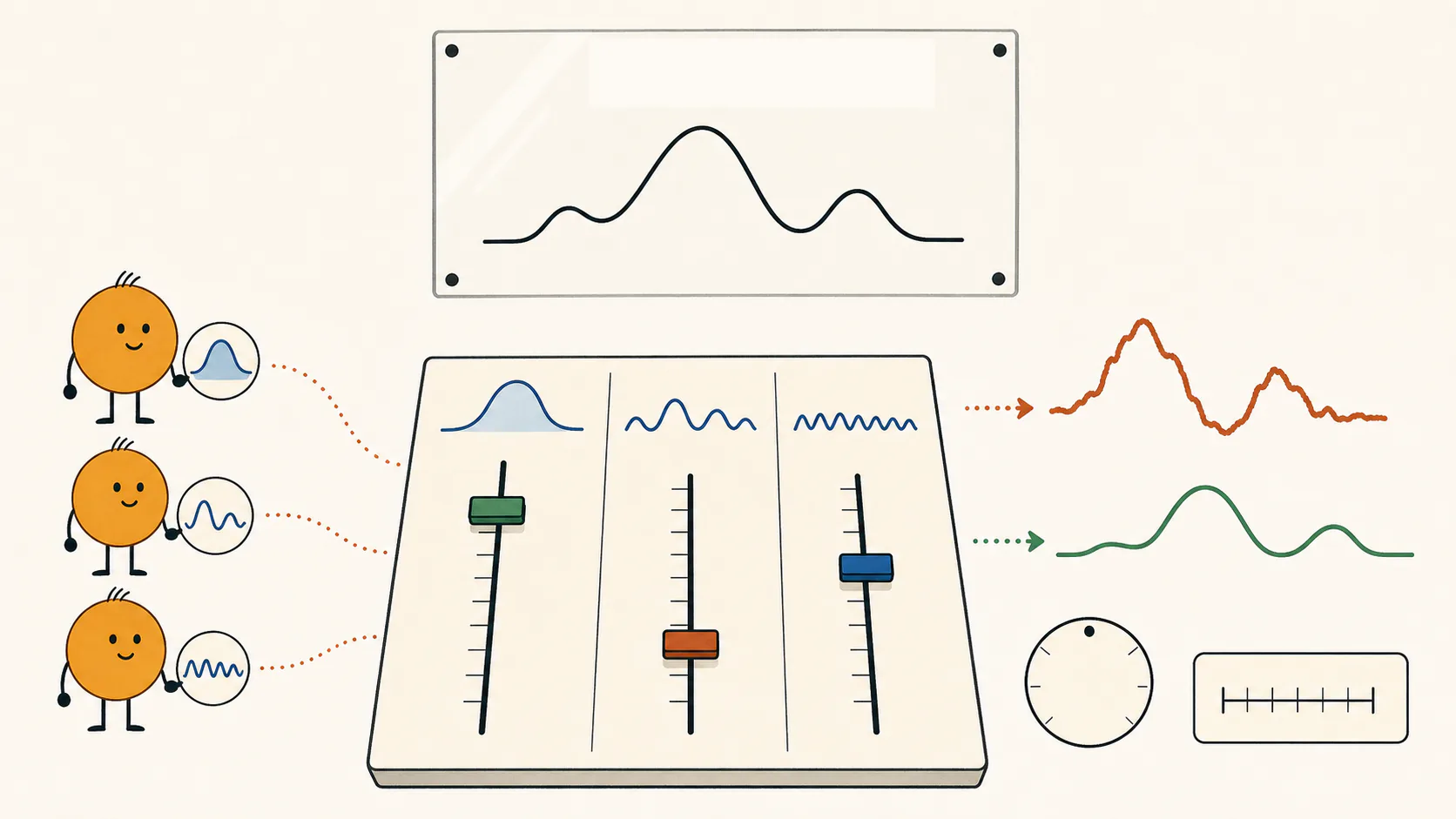
One spike is a volume knob. Several spikes are a mixing board.
Why was one knob enough for one spike? Every piece of the target shared one recovery rate. Give different target modes different spike strengths and that scalar simplification disappears: the learner must recover a shape, not merely set a volume.
Where can several spikes come from? Pretraining across tasksInside: compare joint training with task heads alone, then test transfer to a fixed target
Several reusable directions can become loud together. This small pretraining model shows how that mixing board can arise: fit a family of old tasks, then use the learned representation for a new, fixed target.
The product fits old tasks. Its factorization determines what transfers.
Lift a scalar input into orthonormal Fourier features. The pretraining tasks reuse several of these modes. A shared linear layer A and task heads W jointly fit the fixed task coefficient matrix B.
Two linear layers are redundant: many pairs have the same product. Joint training decides whether recurring modes live mainly in bespoke heads or become loud in the shared representation.
The shared layer multiplies this mode by a; its task head multiplies it by w. Their product aw fits the task. The covariance panel shows a² divided by its average across modes, so its mean eigenvalue stays 1.
At every progress setting, the predictor fits the same selected downstream training labels (four at the opening setting), using minimum-head-norm interpolation. Only the representation changes. Fresh-test error averages the learned green curve’s squared error over a uniform input on [0, 1]. The squared head norm measures the cost of representing the exact gold target in the current features.
Exact solutions for the two training choices
Under this model’s balanced joint population gradient flow, each mode with positive target strength follows an exact sigmoid, a result of Saxe, McClelland and Ganguli (2014).
A physical origin: sensors measure several hidden quantities
A sensor need not measure just one quantity. Let two independent Gaussian physical coordinates Y₁, Y₂ each have variance 1. Let p sensors measure different linear combinations, collected in the response matrix A, with independent Gaussian noise of variance σ². Our fixed target is y = (Y₁ + Y₂)/√2, also of variance 1.
Two shared causes now produce two spikes. Change the sensor responses below: the physical target stays the same, but the two directions can become very unequal in the readings.
What each sensor measures
Two spikes above the noise
Irreducible fresh-test error: (predicting zero scores 1)
Where does that prediction floor come from?
For these Gaussian physical coordinates and sensor noises, the best prediction of y = bᵀY from the readings is linear. Even knowing the sensor responses, its error is
Here the two columns of A are orthogonal. If their full covariance eigenvalues are γ₁, γ₂, the error is ½(1/γ₁ + 1/γ₂). The weaker physical direction can dominate even when the other is measured very well.
The next experiment uses a noiseless target to isolate what unequal feature strengths do to learning. Its scores do not include this physical sensor-noise floor. Continue to the several-spike experiment →
On the SGD page, a first pass at a large rate had a negative-ridge-like bias on a single signal direction. With several directions, one-pass SGD can learn a different gain for each mode. Strong unused modes—amplified directions the target ignores—can make a weak target mode harder to recover.
Changing strengths keeps the target fixed. Switching Fourier/Legendre changes the two-mode target function.
A mode is one basis shape: the cosine with that many cycles in Fourier, or that degree of polynomial in Legendre. The target uses modes 1 and 6; amplified modes 2–5 are unused. Gain is learned amplitude / target amplitude; 1 means full recovery. Scale once and Best in span use true test error. How these gains set the cost of response errors → Dashed mark: Scale once.
| Predictor | Gain 1 | Gain 6 | Training / zero | Fresh-test |
|---|
The live comparison loads with the function.
Changes the experiment to 35 examples; restores Fourier, original strengths/rate, regular-grid samples and shuffled order, then shows the completed pass.
Interpolate
Fit the training targets exactly. Compare both errors; predicting zero scores 1 on each exam.
Scale once
Choose one multiplier for all learned modes. Does it restore both target modes, or does one remain attenuated while the other overshoots?
Best in span
Let the coefficients adjust separately to minimize fresh-test error. Their gains show what one multiplier cannot repair.
One SGD pass
Score the completed pass on your current data, order and learning rate. The live report shows whether it helps here. The explicit 35-example button restores a successful worked example.
Why can one full-batch step work for one signal strength, but fail for unequal strengths?
One gain cannot calibrate unequal signal strengths
From zero, one step of full-batch gradient descent is a scaled matched filter: add the label-weighted inputs, then multiply by one learning rate. For one signal strength, a well-chosen rate can get the signal calibration right in that single step. Give the target two unequal strengths, and the same gain overshoots one component before recovering the other.
This picture shows the mean one-step predictor over independent training sets. It isolates the calibration mismatch; finite-sample variation adds further expected error. The target has variance one, so predicting zero scores one.
Even the best common gain leaves one target component too weak and the other too strong.
The obstruction is to this single matched-filter step. Repeated population-gradient steps can calibrate different modes over time. SGD adds a further question: do its random updates excite strong modes before the weak ones have been learned? The matched pair below tests that question.
What is the matched filter, and what exactly do these curves measure?
Take independent standard Gaussian coordinates sⱼ, signal features xⱼ = √γⱼ sⱼ, and a clean label y = ∑ⱼ aⱼsⱼ, ∑ⱼ aⱼ² = 1. The two-mode examples put half the label variance in each mode; the one-mode example puts all of it in that mode. The strong variance is 100 throughout.
Use the averaged half-squared training loss, start at zero, and take one full-batch step:
That first expression is the empirical label-input cross-moment, multiplied by η. On a fresh input, the mean predictor's coefficient of aⱼsⱼ is ηγⱼ. Each blue bar shows this response; the desired response is one. Consequently,
Minimizing this quadratic over the single shared rate gives
This minimum is zero when all target-bearing modes have the same strength. With unequal strengths and positive target weight in both, it is positive: no common scalar makes both responses one. The selected rate is in units for the averaged loss; using a summed loss divides the same step size by n.
What changes with finite data? Add q independent nuisance coordinates of variance one. For a rate chosen before drawing the Gaussian training set, the exact expected risk of the empirical one-step predictor is
The second term is the prediction cost of sampling variation. Writing Σ = Cov(x) and b = E[xy], Gaussian fourth moments give Cov(xy) = Σ + bbᵀ. Average n independent cross-products and score their variation using Σ to obtain the displayed term. It shrinks with more data. The unequal-strength floor in the plotted mean predictor remains.
Compare full-batch steps with SGD on one spike → See which learning-rate boundary controls which quantity →
How does the exact multispike Pareto frontier allocate training error?
Which mode gets to leave interpolation first?
This three-mode cartoon isolates the lesson of the mixer: the Pareto frontier from interpolation to best in span allocates the allowed training error across modes, instead of multiplying every mode by the same amount. Its widely separated curvature weights make the order easy to see; these are not the mixer’s current settings.
Turning down the common shadow price ω lets us leave exact interpolation and move toward the best-in-span predictor. Coordinate j completes the fraction Aj/(Aj + ω) of that move. Here Aj measures how sharply test error rises when mode j departs from its optimum, relative to the training-error cost of moving it. Larger curvature means more benefit from moving that mode first.
This can matter for classification too: positive rescaling leaves a score's sign unchanged, but unequal mode gains can move its zero crossings.
Fraction of the move from interpolation to the best-in-span predictor
Move right to lower the training-error penalty: x = −log₁₀(ω). On the vertical progress axis, zero marks interpolation and one marks that mode in the best-in-span predictor.
Why one scalar can leave bias
A separate three-mode example. Even the scalar that best removes signal bias leaves the weak modes under-amplified and the strongest over-amplified. These bars stay fixed while you explore the allocation curve.
Exact formula behind this picture
Continue: a matched pair tests what SGD can find →
Can stronger unused features make learning harder?
Can one SGD pass find a predictor as good as the span allows? Try this Gaussian example.
Hold the target, both target-mode strengths, the sample count and the nuisance fixed. Change only the strengths of fifteen other amplified directions, which the label does not use: the unused modes.
Here k=17 amplified directions sit among d total features, leaving d−k unit-variance nuisance directions: the unamplified tail.
A uses the rate rule defined below; B minimizes its expected test error over 80 preset rates. Both rates precede the draw. Best in span chooses weights using the true test distribution.
What changes?
The two gold directions each contribute half of the target’s variance, in both problems.
Bar length shows feature variance. The target and its two gold bars never move; only the unused-mode bar changes.
What stays possible?
The span’s reference interval, from the weaker target mode’s useful-prediction threshold to the stronger target mode’s useful-interpolation threshold, stays put. Only the SGD signal-trace level moves: the total variance of all amplified directions, in units of the weaker target mode’s, tr(Γ)/γk. When it climbs to the sample count, no predetermined constant rate drives the expected one-pass test error to zero.
16training examples
256strong-mode interpolation
4,096
Within that reference interval, both target modes can be predicted before either is learned well by interpolation. The weaker mode's interpolation threshold is farther right, at 65,536. Useful interpolation means good fresh prediction by an interpolator; exact training fit is possible well below this threshold. These are asymptotic reference thresholds, not exact finite-sample cutoffs.
In A, one SGD pass learns both target modes with low fresh error. In B, making the steps small enough to control the strong unused modes leaves the weaker target mode insufficiently learned.
As the family grows, negative ridge drives expected test error to zero in both families. It uses the same samples and is told only the nuisance dimension d−k: no spike strengths, no validation data.
Explore the one-spike ridge mechanism →Same 256 examples, four predictors
Now replace the expectations with one paired Gaussian draw. A/B changes unused-mode strengths while fixing standardized inputs, nuisance, labels and order. SGD also switches from A’s rate to B’s adjusted rate.
| Predictor | Fresh-test error predicting zero = 1 | Training error / predicting zero |
|---|---|---|
| One-pass SGD | ||
| Negative ridge: illustrative shift | ||
| Best in span | ||
| Interpolator |
Active recipe: illustrative shift, fixed before sampling. The conservative spectral margin carries the asymptotic guarantee; choose it above to compare.
The same-draw comparison loads here.
Where does the fresh-test error come from?
Each column splits a predictor’s fresh-test error exactly into the two target modes, unused modes and nuisance; the parts add up before rounding.
| Source | One-pass SGD | Negative ridge | Best in span |
|---|
Which ridge penalty, and what is being measured?
Rows of X are examples, so K = XXᵀ. Negative ridge chooses u = Xᵀ(K + nλI)⁻¹y in the training span. The illustrative penalty is fixed before drawing the inputs:
nλ = (5/2)√(n(d−k)) − (d−k).
We check that the shifted Gram matrix is positive definite before solving; a rejected draw returns zero. This is a finite illustration of the penalty rule above.
For the conservative spectral margin recipe, let d₀ = d−k, z = √(2 log(8n⁶)) and Δ = 2√d₀(√n + z) + (√n + z)². It uses nλ = 2Δ − d₀ only when Δ < d₀/2 and K + nλI ≽ ΔI; otherwise it returns zero. Both recipes use the supplied nuisance dimension and observed Gram matrix, without spike strengths or validation data.
The conservative margin leaves more of the weak target mode unrecovered at this family size. Its guarantee is that expected error vanishes as the family grows; it does not promise the best error on each finite training set.
SGD uses the same rates as the expected errors above: A’s prescribed rate, and for B the lowest expected B-on-B error among 80 preset rates. Both are fixed before the draw. Best in span uses population information. Fresh errors come from the known Gaussian covariance; training errors score these same 256 examples. We draw the nuisance Gram matrix through its exact Wishart law, rather than storing 268 million nuisance coordinates per example.
Continue the SGD inspector’s experiment hereInside: the SGD inspector’s inputs, task and rate; completed errors by mode.
Continue the SGD inspector’s experiment. This panel opens at its default, or at the exact settings carried by a link from it. At the default settings, the standardized draw is the same as the paired comparison above, but the inspector uses slightly distinct unused-mode strengths; the comparison above uses equal strengths within each band. That default difference explains the small difference in their opening errors. The configuration below identifies the spectrum carried by a saved link. The two panels have independent controls.
Open this comparison to calculate its completed predictors.
The original equal-band paired table above remains available. In the distinct default, one SGD pass in A has fresh-test error 0.062591 and illustrative negative ridge 0.081957 on the predetermined draw.
| Learner | Fresh-test error | Training error / predicting zero | Weak | Strong | Other modes | Nuisance |
|---|
Exact expected SGD error: . Across 64 independent training sets:
Follow this same experiment through its SGD updates →
Preserved numerical settings
Displayed settings are rounded for readability; calculations and saved settings retain full precision.
Machine-readable settings
Why can ridge succeed where one pass struggles? Ridge solves for all example coefficients jointly: changing one coefficient can correct its interactions with every other example. SGD fixes each arriving coefficient from the residual at that moment, before later examples have contributed.
While a weak target mode is still being learned, its unfinished residuals drive each update, and each update also writes a random component into the strong unused directions. Because those directions are strong, those random components become large fluctuations in the prediction: that is the variance. Smaller steps keep the fluctuations small, but can leave too little progress on the weak mode in one pass. Negative ridge can make the coupled correction jointly. The full and triangular matrix systems put these coefficient choices side by side.
Both families keep the same 16:1 strengths in the two target modes. Even the best one-step matched filter has error 0.438 in its mean predictor for both: unequal feature variances in the two equally weighted target directions defeat one common gain. Finite-data variation adds error. The A/B contrast instead isolates how strong unused modes obstruct one-pass SGD.
Could one multiplier repair the interpolator? Not in this matched family. Even a multiplier selected with knowledge of the data and the true distribution leaves limiting test error 1/2: bringing one target mode to its target gain leaves the other still short of it. Try “Scale once” in the drawable model above; it illustrates the same shape-versus-volume problem, though it uses different numbers.
What is fixed, and what do the finite runs show?
At M=16, both problems have n=M²=256 training examples, k=M+1=17 amplified coordinates, d−k=M⁷ nuisance coordinates, and target y=(s₁+s₁₇)/√2. The first and last signal variances are M⁴=65,536 and M³=4,096. The fifteen unused directions change from M³ in A to M⁴ in B. Both problems have leading best-in-span test error (M⁻¹+M⁻³)/2≈0.031, and both require large retrospective training loss for accurate span prediction.
The signal-trace level is tr(Γ)/γₖ: 32 in A and 257 in B. In the separate 64 paired equal-band Gaussian draws at M=16, A's prescribed one-pass SGD rate had median test error 0.064. B's lowest median across 92 tested constant rates was 0.208. That grid is finite; the theorem covers every predetermined positive constant rate in B and rules out vanishing expected test error for all of them. The negative-ridge predictor with the conservative spectral margin attains vanishing expected risk in both families; B has not lost its good span predictor.
Is B just a harder exam?
Train on A or B for one SGD pass, then freeze the predictor before choosing where fresh test inputs come from. The values below average over training draws. Start with the same M=16 family as above, then grow it.
One trained predictor, two tests
A uses its prescribed rate; B uses the rate that scores best when trained and tested on B, chosen from a fixed sweep.
It adds the expected error in the two target modes, unused-mode error and fresh nuisance error.
- Expected error in the two target modes
- Unused-mode cost
- Fresh nuisance error
What happens as the family grows?
Expected test error, log scale. The dotted line is B → A's asymptotic lower bound, e^-4/2 ≈ 0.0092. Grow the family to M=64 to see the crossed evaluations swap order; the theorem concerns their limits.
At M=16, A-trained SGD already beats B-trained SGD on B's own exam: 0.141 versus 0.216. Grow the family: A-trained SGD eventually succeeds even on B, while B-trained SGD at any predetermined constant rate retains a risk floor even on A. The obstruction is in the training updates, not merely in the exam.
What is fixed, and how are these risks computed?
The two populations have the same label rule and true linear predictor. Only the variances of modes that carry none of the label differ. For any fixed predictor, testing under B adds exactly
These are exact Gaussian expected risks from the four-component one-pass recurrence, not individual simulation runs. A uses its prescribed rate eta_A = log(M)/(2M^5) ( here). For B, we choose the lowest B-on-B expected risk among 80 logarithmically spaced rates with n eta M^3 in [0.001, 2.5] ( here). That B rate stays fixed when its predictor is tested on A. This finite search illustrates the result; the asymptotic multispike lower bound applies to every predetermined positive constant rate, not just those 80.
Under A's training law, weights learned on the unused modes become small enough that even B's heavier test weighting has vanishing cost. Under B's training law, making the step small enough to control all those strong modes leaves residual error in a weak target mode. Testing on A removes the extra unused-mode penalty but cannot undo that missed learning. This does not claim the same floor for other estimators or arbitrary learning-rate schedules.
You have the main story.
A learned function can recover the target while badly answering its own training points. With unequal signal strengths, recovering the shape takes more than a common rescaling. One-pass SGD can learn that shape, but holding strong unused modes in check can leave weak target modes unrecovered. In the matched families above, negative ridge still drives expected test error to zero in both as the family grows.
Continue to Oja without labels, or change one more ingredient below:
- Fourth moments: keep covariance and learning rate fixed, then see why Gaussian and uniform inputs can make expected SGD error grow or shrink.
- Watching runs: compare strict and tolerant checks on held-out examples, and see when a monitor rejects useful learning.
- Nuisance spectrum: concentrate the same variance in fewer frequencies and watch the narrow training-point corrections spread.
Explore fourth momentsInside: hold covariance fixed and compare expected error, typical runs and raw inputs
Same covariance. Same learning rate. Same fate?
Not necessarily. A single SGD update multiplies coordinates together, so its stability can depend on fourth moments that the covariance does not record. A standardized coordinate’s fourth moment is its average fourth power, which gives unusually large arrivals much more weight. This example removes nuisance entirely: ten strong unused modes compete with one weak target mode. Any failure below happens among the amplified modes themselves.
The gold target stays y = s₃. At this setting, Gaussian amplifies (factor 1.02 > 1) while standardized uniform contracts (factor 0.989 < 1).
The vertical scale stays put: a runaway curve runs off the plot, and the corner label gives its largest value.
This draw is one path, not the expectation. The comparison below shows how variable those paths are.
At the opening setting (G = 4, η = 0.04375), click Jump to 300.
1. Same covariance: compare Gaussian with Uniform. Do their expected test errors end the same way?
2. Mean versus typical run: choose Fourier lift. Compare the expected test error with the median, then look back at the Fourier paths above.
3. Same expected curve: choose Sparse code and Match Gaussian fourth moments. Does matching the mean also match the typical run?
These settings also update the Fourier view above.
For the selected input law, exact expected test error averages over training draws. The empirical median is the middle of 180 simulated runs; the shaded middle 80% shows how widely those runs vary.
The stability boundary is near 5.0 nonzero coordinates on average. The ruler below compares the fourth moments of these sampling laws.
The mean-square factor describes long-run growth or decay of expected squared error; individual runs can vary.
Cell height is magnitude; blue is positive and rust is negative. Hover a cell for its value. The covariance is identical across tabs, but the joint patterns are visibly not.
Gaussian draws have all 11 coordinates nonzero. Standardized sparse codes with 3.67 or 6.11 nonzero coordinates on average match the Gaussian or standardized-uniform fourth moment, respectively. For these independent symmetric coordinate laws, matching that moment matches the expected SGD recurrence. Fourier has additional mixed fourth-order terms, so it cannot be placed on this one-number scale.
Exact model and numbers behind this comparison
Explore monitoring a runInside: compare strict and tolerant checks with a smaller learning rate
Train a linear predictor of y=s₃ from eleven features: the target feature has variance 1 and the other ten have variance 4. The target, feature variances, and 300-example budget stay fixed across input-law tabs; ordinary SGD uses learning rate 0.04375, while “Smaller step” uses 0.03.
Reserve a few examples and reuse that same monitoring set after every block. Offer the remaining examples to SGD in blocks of ten ordinary sequential updates. After each block, the monitor decides whether the proposed checkpoint survives. A rejected block still consumed its examples and computation: rollback is not a refund. The sparse input law matches Gaussian fourth moments: each standardized coordinate has fourth moment 3.
Same 300 distinct examples in total. Unguarded SGD and Smaller step use all 300 for gradient updates; guarded methods reserve h for monitoring and train on the remaining 300 − h.
These comparisons concern the displayed rules, laws and budgets. Rejecting temporary increases can reject useful learning; they do not establish that all monitoring fails.
No training block has been offered yet.
Large runs sometimes restore an earlier checkpoint and continue past a loss spike with different data. The PaLM training report describes checkpoint-and-skip interventions and notes that implicated batches did not reproduce the spike from a different earlier state. This toy does not explain PaLM. It gives us a tiny system in which the same state–data interaction can be inspected rather than merely survived.
What did the monitor see?
Dots mark accepted blocks in green and rejected blocks in rust. Monitoring loss chooses; test error scores the decision afterward.
In this eleven-dimensional clean model, the monitoring loss is (u − e3)TQmon(u − e3), where e₃ is the target predictor y=s₃. Five monitoring points leave unseen directions. Twenty Gaussian points usually span all eleven, but can still measure some directions poorly. Reusing the monitor is therefore part of the algorithm, not a free independent audit.
Exact protocol and numbers used in this experiment
Explore the nuisance spectrumInside: move the same nuisance variance into fewer frequencies
What if nuisance is concentrated in only a few directions?
The narrow nuisance corrections could be large at training points while leaving most fresh inputs alone. Now hold signal strength and total nuisance variance fixed, but concentrate the variance in fewer Fourier modes. This separate experiment uses a constant target and nine training points, evenly spaced or drawn uniformly on [0, 1]. Watch how the corrections spread.
Signal strength 99; 1,188 Fourier nuisance features sharing total variance 1,188. Each frequency has two features, sine and cosine: the concentrated preset keeps 27 frequencies, or 54 features. The nine training locations stay fixed as you change the spectrum or predictor.
The thresholds mark gradual changes in prediction quality. In the balanced grid comparisons, best test error is n_useful/(n+n_useful), where n_useful is the useful-prediction threshold. At the 54-feature endpoint, nine samples give fresh-test error 0.23 and old-input loss 0.64: this best-in-span predictor beats predicting zero on both exams, even with n between the markers.
The markers summarize the feature spectrum. The curve, both heatmaps and both errors are recomputed at your nine drawn locations.
Where the input variance lives
Best in span: learned Fourier power
Recovered signal (0 Hz): gain —; power —. Black mark: target power 1.
One trip around the circle is one second, so the harmonics have integer frequencies in Hz. Both axes are compressed but include zero; ticks give the actual frequency, variance or power. Each nuisance bar combines the sine and cosine at one frequency. Gold shows the signal direction's variance on the left and its recovered power on the right.
Concentrate the same nuisance mass into fewer modes. The narrow interpolation lobes can spread into the gaps between points. The best-in-span predictor recomputes the best whole function, not merely its overall height.
Total nuisance variance describes the features. The reported nuisance energy measures the nuisance in the learned function on fresh inputs.
Two effective ranks summarize how that nuisance variance is distributed.
How large is the remaining spectral mass compared with its tallest nuisance direction?
How many nuisance directions are effectively sharing that mass?
Sampling contributes one copy of the nuisance spectrum; fresh evaluation contributes another.
These effective ranks were developed by Bartlett, Long, Lugosi, and Tsigler (2020); the subscript 1 sets the spike aside, so both ranks describe the nuisance tail. Here total nuisance variance stays fixed, so the interpolation threshold stays at 12. Concentrating that variance increases the squared spectral mass and moves the useful-prediction threshold to the right. Mass-to-peak also helps diagnose when the scalar-Gram approximation is reliable; it is not a separate dial for either threshold.
Here the observed nuisance vectors are the columns of Z. Both heatmaps are in sample space: row i and column j identify training examples. The sample Gram is divided by total nuisance variance; the fresh-test Gram by the sum of squared nuisance variances. Colors saturate at −1: rust and +1: blue; 0 is white.
Why are there two Gram matrices?
Did the two rulers just swap roles? No. There are two different matrices. Ω is covariance in nuisance feature space. W = ZᵀZ is the Gram matrix of the observed nuisance vectors, in sample space.
Fresh nuisance risk is α⊤Z⊤ΩZα. Training's nuisance self-response is α⊤W2α/n. When Ω = I, fresh risk reduces to one copy of W, exactly as in the stylized model. A nonflat feature spectrum adds a new weighting to fresh risk; it does not remove training's extra Gram factor.
Every high-frequency Fourier coordinate is scaled by the square root of its displayed eigenvalue. The low-frequency signal and the target function do not move. The second heatmap uses the squared eigenvalues because a fresh covariance-matched test point supplies another copy of the nuisance covariance.
Exact spectral dictionary and displayed numbers
Continue: Oja without labels →Return to the short-route takeaway ↑