Can a list of numbers teach a shape?
Run one pass, then raise the spike strength. Compare Oja with batch PCA on the same consumed examples. Neither method sees target labels. Changing the input density changes what direction there is to discover.
stream begins after the first sample
The rust curve evaluates Oja’s current direction at each input. Drag the white diamond sideways to inspect a value and pause the movie, or use the input slider below the curve. Vertical swipes scroll.
The white diamond uses the full weighted sum, including all the remaining coordinates.
Log scale: at 1 the spike is no stronger than a nuisance coordinate; 180 is a strong spike.
Try Full pass → fit fresh labels → γ = 30 → fit fresh labels again. Both examples use the same inputs and order; the radius view keeps the benchmark.
Consume unlabeled inputs, then . Only these labels choose the scale; the two exams below use the old inputs and independent uniform inputs.
Benchmark until you draw fresh labels
The same calibrated predictor is scored on fresh inputs and the consumed prefix.
The nuisance component is scored on these same two exams.
Compare one fresh label with three →Why can old inputs score worse? They helped choose the direction, so it still carries some of their nuisance. Scored on those same inputs, it meets that stored nuisance again. On uniform fresh inputs the same nuisance is averaged over the whole domain instead.
Before calibration, the cards show the test-optimal benchmark, using true population risk. Afterwards they show the learned scale. Predicting zero has fresh error 1.
Total error also includes missed signal and, on old inputs, its cross-term with nuisance.
Direction sets the learned shape. Display normalization gives the Oja, PCA, and population-mode shapes mean square 1 under uniform inputs, with signs oriented toward the spike. Calibration chooses a multiplier for prediction.
Direction diagnostics before calibration
Predictive correlation²: learned score versus the label on uniform fresh inputs. For Smooth mix, green-mode overlap² compares the learned function with the green population-mode function, also under uniform inputs.
How one number becomes one point on the curve
Follow the latest input through the fixed lift and the movie’s current direction weights.
white diamond on the rust curve
See the products and the rest of the sum
| Coordinate | Feature φⱼ(x) | Weight wⱼ | Product |
|---|---|---|---|
| Remaining coordinates, summed | 0.000 | ||
Oja’s curve is linear in these fixed features, even when it wiggles in the input.
Where is this experiment relative to the two finish lines?
How differently do Oja and PCA weight the same examples?
Batch PCA is hidden in “Oja only” mode. to compare how they weight the same examples.
Each bar is a signed coefficient multiplying one consumed input’s feature vector. Oja’s bars and PCA’s bars are each divided by their own largest absolute coefficient; their heights compare relative weights, not absolute magnitudes.
What else can I try?
What changes when I redraw the inputs? Uniform random locations change the Gram geometry as well as the arrival order. The darker stems still show arrival time, but their lobes now overlap; on the grid they barely interact.
Can the dominant mode differ from the spike? Choose “Smooth mix.” The black curve is the fixed spike reference; thin blue shows how much of it is present in the current Oja estimate. Green is the leading population eigenfunction of the full uncentered second moment. Watch whether rust approaches green.
Why does the green curve move with spike strength? The feature map and the input density jointly determine the second moment. Changing a feature's weight can therefore change the leading eigenfunction, not just its eigenvalue.
Is the Fourier basis essential? Switch to Legendre. The shapes and Gram interactions change, while the competition between signal growth and accumulated nuisance remains.
What are the coefficient bars saying? Normalization attenuates older contributions. In the orthogonal preview that produces an exact geometric recent-sample window; in the random stream it is a guide to the realized weights, not a literal count.
What is exact here, and what is interpretive?
Here Oja and batch PCA use the uncentered second moment M = E[φφ⊤]. For uniform inputs these features have zero mean, so this is also their covariance. For the smooth mixture they do not: we do not subtract the mean. That distinction matters when the green population mode changes.
The Fourier playback recomputes the Gram matrix from the actual locations and finite feature lift. Batch PCA is the leading direction of the uncentered empirical second moment on exactly the displayed prefix.
The smooth mixture is a separate finite experiment; it uses the same fixed lift and exact finite Oja updates. We drew its centers and weights once and kept them because they give a visibly informative top mode; Gaussian blurring gives a continuous distribution, with zero probability of any one exact input.
The formula relating each nuisance lobe to its age requires complete Fourier alias blocks. Here 630 frequency pairs do not divide into 100 grid points, so even the grid retains nonzero nuisance interactions. The participation figure is an orthogonal-model comparator, not the measured effective sample count. Legendre also uses its exact finite Gram matrix.
Exact formulas used in this playback
The finite playback uses each actual feature vector and Oja update. It compares the resulting direction with batch PCA on those same consumed inputs; fresh scores average over uniform inputs. The settings and detailed calculations below preserve the full numerical record.
Exact settings, formulas and numerical values
What do labels buy? Compare with batch PCA.
Without labels, PCA must discover the predictive direction from covariance alone. Can a streaming method recover a direction that is already useful for prediction, without ever forming the batch covariance matrix? The first landmark below is the Baik–Ben Arous–Péché (BBP) threshold: the point where ordinary batch PCA first gains nonzero population alignment with the hidden spike.
Squared predictive correlation
Spike strength gamma
For the mathematically curious
Let h be squared Euclidean overlap with the spike, and let casp = (d−1)/N = 4. The best scalar calibration converts overlap into squared predictive correlation:
In the fixed-aspect Gaussian limit, PCA has squared Euclidean overlap (for γ > 1)
Substituting this overlap into the calibration formula cancels its denominator. The two metrics differ: modest directional alignment can support much stronger predictive correlation.
For the best predictor in the labeled span and for PCA, respectively:
The PCA expression applies above γ = 1 + √casp; below that threshold its predictive correlation is zero. Here (z)₊ = max(z,0).
Exact parameters and numerical values
What is the BBP threshold doing in this story?
To the left of the line, the leading empirical eigenvector cannot reliably tell which way the spike points. To the right, covariance alone starts to reveal it.
Labels change the game: each labeled example carries a hint about which direction is predictive. That is why supervised prediction can become useful before PCA’s direction has lined up with the spike.
The movie asks a more algorithmic question: can one-pass Oja reach that useful region, where a direction predicts well while still overlapping the spike only weakly, from a stream of unlabeled examples? For a strong spike, the Gaussian one-pass result gives a yes: the same polynomial sample count as batch PCA, up to logarithmic factors.
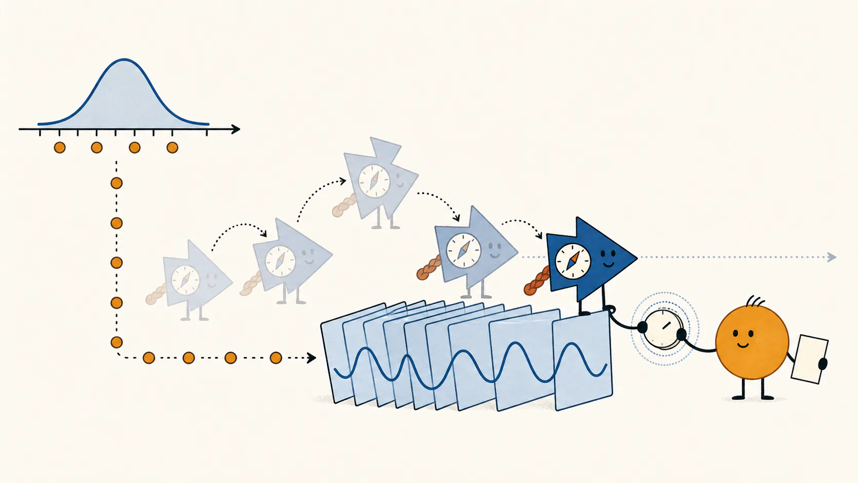
Take (most) labels away.
The unlabeled pass learns a direction. A tiny fresh labeled step afterward chooses the scale needed for prediction.
Scrub across either plot, or use the sample-count slider.
Formulas used in this high-signal picture
Define the high-signal detection and strong-recovery parameters, then compute the batch-PCA overlap h:
Calibrating this direction using the true test error gives
The high-signal approximation replaces γ−1 by γ in both parts of the BBP overlap formula above; the calibration formula remains exact for a given overlap. The Gaussian one-pass analysis matches these sample-count orders up to logarithmic and confidence factors away from the thresholds.
Exact parameters and numerical values
Why are there two finish lines?
Between these thresholds, calibration can make prediction useful while the direction’s Euclidean overlap is still small.
Past the first finish line, the learned direction carries some of the spike, and a scalar can calibrate it into a predictor that beats predicting zero. Past the second, the direction itself lines up with the spike: its Euclidean overlap², the squared cosine between the two in raw coordinates, becomes substantial; near-exact recovery needs sample counts well beyond it. The ledger’s predictive correlation² is the squared correlation between the learned direction’s score and a fresh label; it equals one minus the test error at the test-optimal scale.
With total input dimension d and one signal coordinate, there are d−1 nuisance coordinates. For a strong spike, the detection threshold (the first finish line) sits at s2 = γ2N/(d−1) ≈ 1. The exact fixed-aspect BBP boundary uses (γ−1)²N/(d−1) = 1; this high-signal picture replaces γ−1 by γ. The ratio ρ = γN/(d−1) measures N against the strong-recovery threshold (the second finish line): ρ = 1 is that line, and recovery becomes near-exact only well beyond it, for ρ ≫ 1.
Between them, Euclidean overlap can still vanish. But prediction cares about predictive signal-to-noise, which receives an extra factor of γ: a direction at angle θ to the spike, at its test-optimal scale, has test error tan²θ/(γ+tan²θ), small once γcos²θ ≫ 1 even when the overlap² cos²θ is tiny. A direction with little Euclidean overlap can therefore make a strong predictor after scalar calibration.
Initialize from one consumed sample. That buys a factor-of-γ head start over starting from a random direction.
Score the next feature vector in the stream against the direction found so far, then use that score in the update: w ← w + η (w⊤φ) φ, followed by rescaling w to unit length.
Fresh labels choose the scale on the learned line. In the Gaussian model, once the direction is well learned, one fresh label works with high probability, and scalar least squares on three fresh labels also controls the expected test error.
With one fresh Gaussian label, calibration divides by a score that can happen to be almost zero. Least squares with three fresh Gaussian labels tames that small-denominator tail.
Exactly what do three labels buy in the Gaussian model?
With one fresh Gaussian label, if the learned direction still carries nuisance, that small-denominator tail makes the expected test error infinite.
Freeze a nonzero direction independently of the fresh calibration examples. Let Roracle be its best population error after scalar calibration. Fit a scalar by least squares through zero on m fresh Gaussian examples. Averaging over those calibration examples gives
Three labels give twice the oracle error in expectation. With one or two, the expectation is infinite whenever Roracle > 0. This Gaussian identity explains the label count; the Fourier and Legendre experiments use uniform inputs and compute their actual errors separately.
The labels are new to the predictor; the inputs are not.
The old inputs’ labels score the predictor; they never taught it the direction or chose its scale. In the Gaussian benign-misfitting window, the calibrated predictor can pass the fresh-input exam and fail this old-input one.
Detected, aligned, or actually consistent? The scholarly gap between two spectral finish lines.
A thoughtful reader may object that “PCA found the spike” hides several different claims. The BBP transition asks when the leading empirical direction first separates from the noise bulk and gains nonzero information about the population spike. That is detection, not full recovery. There can be a long middle in which the empirical direction has a useful signal component but still carries a substantial random completion outside the spike.
Wang and Fan’s analysis of empirical eigenvectors makes that middle geometrically concrete: in their high-dimensional spiked setting, an empirical eigenvector can look like a deflated population direction plus a random component in the nonspiked coordinates. Consistency arrives only when the relevant dimension-to-sample-and-spike ratio vanishes. That is the right scholarly neighbor for the weak-overlap window in the animation above: not “PCA failed,” and not yet “PCA recovered the direction.”
The precise assumptions and boundaries differ across fixed-aspect BBP asymptotics, growing-aspect eigenvector asymptotics, and the one-pass Oja result. What survives the translation is the useful distinction between first visibility and consistent recovery.
Oja learns a line. A label chooses a point on it.
The movie fixes the function's L² norm to compare shapes. But a regression predictor also needs a scale. Keep the direction you just learned and ask how far to move along it.
The guide changes scale while keeping the learned direction fixed.
Connect the movie direction to compare both scores.
The best radius stops short of unit survival because a little missed signal can be cheaper than amplifying all the nuisance attached to the direction. Change the movie's spike strength or stream and the ray tilts with its learned direction.
Can covariance stretch a poorly aligned direction into a useful predictor? Compare Euclidean overlap², the squared cosine between the learned direction and the spike in feature coordinates, with Predictive correlation², the squared correlation between its score and the label on uniform fresh inputs.
Signal survival r: the selected predictor’s spike coefficient; 1 restores the target.
Movie normalization
The movie fixes a norm to compare directions. Score that normalization as a regression predictor on the current ray. Its test error is the sum of the two squared costs beside the plot.
Test-optimal scale
Choose the point on this ray with the smallest true fresh-test error. Restoring every bit of signal can cost too much nuisance. Compare squared missed signal with squared nuisance contamination.
Unit signal survival
Restore the signal coefficient to 1. Missed-signal error becomes zero, but the direction still carries nuisance; read the cost of amplifying it.
Let fresh labels choose
The benchmark above uses the true test error. Inspect the current direction with one or three fresh labels to estimate its scale.
Let one or three fresh labels choose the scaleInside: freeze a direction, then compare one-label and three-label fits.
One or three fresh labels. One frozen direction.
The opening procedure freezes Oja’s feature-weight vector u with Euclidean length 1. Its score is g(x) = uᵀφ(x). Draw three fresh uniform inputs and their labels. Fit the first label with c = y / g(x), or use all three with scalar least squares: c = ∑ g(xj) yj / ∑ g(xj)2. Both choices use the same fresh set and frozen direction; only these labels choose the multiplier.
The movie uses a different normalization: it divides this score by its RMS under uniform fresh inputs, and orients its sign toward the spike. If a is the frozen score’s spike coefficient and q = √E[g(x)²], the movie shows coefficient |a|/q, while calibration gives signed signal survival r = ca.
Three scales on this frozen direction
Signed signal survival r: 0 predicts no signal; 1 restores the target.
Fresh-label-scaled predictor: scored below on the same two exams, with predicting zero as the reference.
The first draw freezes the current movie direction and its consumed inputs.
Draw a fresh set, then compare one-label and three-label calibration.
A tiny score can make one-label calibration choose a huge multiplier. In the named example, fitting all three nested labels repairs it; redraws need not favor three. Fourier nuisance sits in narrow lobes, which a few calibration points can miss. The Gaussian expectation result above is a different calculation.
One pass was the deal. Does reversing the stream make Oja forget?Inside: compare replay in the same order with replay in reverse.
Late samples retain much larger coefficients than early samples. Replaying in the same order begins with the heavily attenuated early points, which partly shields the direction. Reverse replay begins with the loud, recently seen points and can rotate the direction abruptly.
This is an empirical diagnostic. Reducing the step after the first pass often softens the boundary shock. The exact one-step rotation depends only on the current score and the sample component transverse to the current direction.