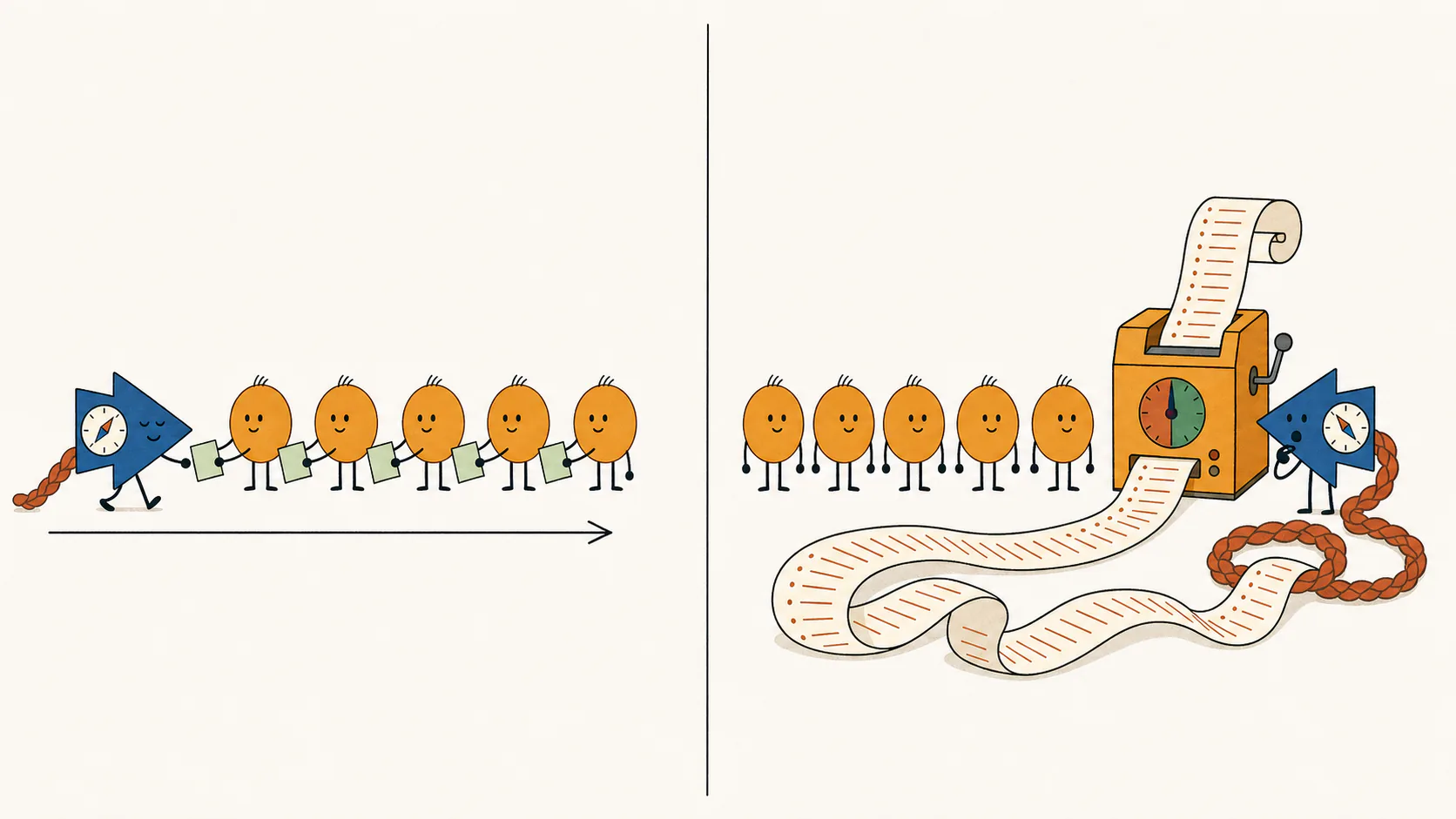
One-pass SGD
Replace the diagonal by 1/η. Mask future comparisons with zeros.
| 1/η | 0 | 0 |
| K₂₁ | 1/η | 0 |
| K₃₁ | K₃₂ | 1/η |
If the first epoch helped, why not run another?
In the default stylized run, one pass lowers fresh-test error to 0.0672 while training error climbs to 23.7 times predicting zero’s. On the first return, fresh-test error jumps to 0.216; after three passes it reaches 206. Returning points find their own nuisance in the predictor. The rate that recovered the shared signal feeds that nuisance back into learning.
If you landed here first: Benign misfitting means predicting fresh examples well while fitting the training examples worse than predicting zero.
SGD—stochastic gradient descent—adjusts a predictor using one labeled example at a time. Its learning rate η sets how large each adjustment is. In the Stylized and iid models, each label is the exact signal coordinate. Nuisance is the unamplified part of the input; it does not enter the label. Use the controls above the plot to compare Stylized examples with separate nuisance directions, an independent and identically distributed (iid) Gaussian draw using Make iid, or a noisy sensor rack using Sensor style. Sensor style uses the Sensors page’s opening rack; follow it on the Sensors page.
The green curve scores fresh inputs; the rust-colored curve scores all 100 training points using the same current predictor. Both start at 1. Choose First update to see how the separation begins, then End first pass and First return.
In the Stylized and iid models, the signal strength is γ = 100, the total input dimension is d, the number of nuisance coordinates is d−1 = 50,000, and the target is y = x[1]/√γ. Both error curves start at 1 for predicting zero.
In stylized mode, training example i is xi = √γ e1 + √(d−1) ei+1, with label 1. These are deterministic, orthogonal nuisance vectors, not an iid Gaussian training draw. A fresh input has covariance Σ = diag(γ, 1, …, 1).
In iid mode, each label is an independent standard Gaussian, and each input has signal coordinate √γ times its label plus 50,000 independent standard Gaussian nuisance coordinates. The dataset stays fixed as you change the learning rate or press Play again; New iid draw generates another dataset. The full training curve is divided by that dataset’s mean squared label, so predicting zero scores 1 on it. Losses before each update and the point scorecard show raw squared losses.
Sensor style uses 100 independent calibration examples and 50,000 sensors, each with noise variance 500. The label is the physical quantity Y; every sensor measures it with independent Gaussian noise. Training error is divided by this rack’s squared calibration labels, so predicting zero scores 1. Fresh error averages over new physical quantities and sensor noise.
We use the half-squared-loss update u ← u + η(yi − ⟨u, xi⟩)xi, the least-mean-squares (LMS) rule of Widrow and Hoff (1960). The factor ½ cancels the 2 from differentiating the squared residual, fixing what the learning-rate numbers mean.
Follow four stops: first update, end first pass, first return, then end third pass. The guide uses your selected model, rate, data and order.
At the opening rate, fresh-test error is 0.0672 after one pass, 0.216 at the first return, and 206 after three passes.
100 examples; orthogonal nuisance; exact labels
“Best one-pass rate” uses the true test error to choose the rate, information unavailable from the training examples alone.
Viewing end of pass 3 (update 300).
After each update: population fresh-test MSE and mean training MSE on all 100 examples, divided by that dataset’s mean squared labels.
Stylized inputs contain the clean target coordinate. Population test error can reach zero if that direction is known.
Remaining signal error Its stored nuisance Residual on return
Stored nuisance is the sum of:
One example changes the predictor. Both curves score the predictor after this update: one on fresh inputs, the other on the entire training set. Read both errors at the selected learning rate.
Each point has been used once. Compare the two errors for your current run. At the opening Useful first pass rate, fresh prediction improves while training error climbs; a gentle rate can behave differently.
This point encounters nuisance already stored during learning. The ledger subtracts stored nuisance from remaining signal error. In iid data, the contributions from other points can have either sign.
The same examples have been used three times. Compare these two errors with the first-pass stop. The opening Useful first pass rate fails under reuse; your selected rate determines what happens here.
During the first pass, the arriving point has not contributed its own nuisance yet. In Compare curves and losses just below the plot, choose Each point before its update to see each raw observation, and Moving average of these losses to reveal the trend. In the iid first pass the dots fluctuate: each point is one noisy observation of the current predictor’s quality, even though its label is exact. Evaluating the current predictor on all 100 training points asks a different question from evaluating the next point before its update, the fresh-stream question of Robbins and Monro (1951).
For a fresh iid example independent of the current predictor, yes in conditional expectation: its squared loss, measured before the update, has expectation equal to the current iterate’s population test error.
In the Stylized (deterministic cartoon) setting, the arriving nuisance direction is exactly orthogonal to every earlier one. Its first-pass loss is just the squared signal bias. Fresh Gaussian test error additionally includes the accumulated nuisance energy, so the two plotted quantities need not coincide. Both can be small while retrospective training error is large.
At the same numerical learning rate as useful SGD, full-batch GD steadily fits the training set. At a much larger rate, its very first step predicts well—and continuing ruins it. This comparison uses the stylized model: 100 examples, signal strength 100, and 50,000 orthogonal nuisance coordinates.
One full-batch step averages the gradients of all 100 examples. One SGD step uses just one example. The horizontal axis below counts batch steps.
Learning rate η = 0.01; the full-batch stability threshold is 0.003333.
Because the batch gradient is an average, giving each example gradient the same weight as an SGD update takes a batch rate 100 times larger. The batch computes all 100 gradients at one frozen predictor; SGD recomputes the gradient after each point changes the predictor.
The first step gets the signal response exactly right. The same predictor does 20 times better than predicting zero on fresh inputs and 25 times worse on its training set.
The one-step success uses a single signal strength. A full-batch step from zero is a scaled matched filter: average each input times its label, then multiply by one rate. That one multiplier can calibrate this signal. Two unequal signal strengths generally demand two different multipliers.
Write L for the average squared training error. We take gradients of L/2, the averaged half-squared training loss. The reported errors omit the half, so predicting zero scores 1:
L(u)/2 = ‖Xu − y‖²/(2n); uₖ₊₁ = uₖ + (η/n)Xᵀ(y − Xuₖ).
Starting from zero gives u₁ = (η/n)Σᵢyᵢxᵢ. Every stylized label is 1 and each input shares the same signal coordinate. The first step’s signal response is r₁ = ηγ. Thus η = 1/γ calibrates it exactly; averaging the separate nuisance directions leaves test error (d−1)/(nγ²) = 0.05.
All batch iterates give equal weight to the examples. Write rₖ for their signal response: a value of 1 means correct signal calibration. Both errors follow from that one number:
Test error = (1 − r)² + (d−1)r²/(nγ²); training error = [1 − (1 + (d−1)/(nγ))r]².
The next batch step sees the stored nuisance too. Its exact recurrence is
rₖ₊₁ = [1 − η(γ + (d−1)/n)]rₖ + ηγ; r₀ = 0.
At η = 0.01, the multiplier is −5. The first response is 1; the next is −4. Fresh-test error jumps from 0.05 to 25.8. Batch convergence instead requires 0 < η < 2/(γ + (d−1)/n) = 1/300. Within that range, the iterates approach the interpolator: training error vanishes, but fresh-test error tends to about 0.696.
Removing the average from the loss multiplies its gradient by n; matching these updates then requires dividing the learning rate by n. Compare these batch thresholds with population GD, fresh SGD, and the residual on one selected example.
The live iid mode above uses the same signal strength, dimension, and sample count as the stylized experiment. A separate Gaussian experiment tests a larger multispike model across 64 independently drawn training sets of 256 points. Its archived results show median fresh-test error falling while median full training loss rises.
Follow the 100-point run selected above. Each update leaves a track in the predictor: a weighted copy of its input vector. On return, a point is tested against its own earlier contribution. That self-comparison can turn a small remaining signal error into a large residual with the opposite sign. In iid data, the nuisance left by other points also contributes; it can be larger than the returning point’s own track.
The noisy-sensor experiment gives a physical version of this self-comparison. Its correlator weights each sensor by what it read in one reference reading, divided by the known total response energy p, and never changes afterwards. Let N₀ᵢ be sensor i’s noise in that reference reading, and Nᵢ its noise in a fresh reading. Fresh sensor noise gives products N0iNi with mean zero; reusing the reference readings gives noise squares N0i2 instead.
Inspect this run’s first-return ledger beside the loss plot.
A returning point encounters the tracks already laid down.
Two different constraints compete. A small step treats each individual point gently, including on its first visit. A larger step can recover the shared signal much faster, even while overshooting the point it just used.
Shuffling changes which track gets hit next. It does not erase the tracks.
In the stylized model, the gentle rate and the same order each pass eventually fit all 100 points exactly: the predictor approaches the minimum-norm interpolator. Training error goes to zero, but fresh-test error levels off near 0.696—far above the useful first pass.
Starting with a large pass does not change this limit: subsequent passes at the displayed gentle fixed rate, continued to convergence, reach the same minimum-norm interpolator.
| Predictor | Fresh-test error | Training error / predicting zero |
|---|---|---|
| Gentle on each point · first pass η = 10⁻⁵ | ||
| Limit of repeated gentle passes Same rate and order · minimum-norm interpolator | 0 | |
| Useful first pass η = 2 × 10⁻⁴ |
In the multispike high-dimensional limit, where interpolation does no better than predicting zero, any number of gentle steps from zero leaves test error near that baseline. Every step from zero adds a multiple of a training input, so SGD stays in the training span. The Why the Span? page explains why combinations of the observed examples constrain what the learner can recover.
On its first visit, a point is compared only with points that came before it. On its return, the comparison includes an earlier copy of itself.
Each coefficient αᵢ weights training example i, rather than feature i. Adding the weighted input vectors produces the predictor’s feature-weight vector. Collect the input comparisons in the Gram matrix. Each entry measures how strongly two inputs line up: shared signal plus any shared nuisance. A diagonal entry compares a point with itself, so its nuisance part is much larger than the off-diagonal nuisance. One-pass SGD replaces that observed diagonal with 1/η, the inverse learning rate, and masks the entries of points that have not arrived yet. Ridge adds a penalty to the observed diagonal and keeps both triangles. This triangular reading of one sweep is classical: Elfving and Nikazad (2009), with a later treatment by Elfving (2025); Liu and Príncipe (2008) give the same online coefficient reading for kernel least-mean-squares (LMS).
Replace the diagonal by 1/η. Mask future comparisons with zeros.
| 1/η | 0 | 0 |
| K₂₁ | 1/η | 0 |
| K₃₁ | K₃₂ | 1/η |
Shift the diagonal by nλ. Keep both triangles.
| K₁₁ + nλ | K₁₂ | K₁₃ |
| K₂₁ | K₂₂ + nλ | K₂₃ |
| K₃₁ | K₃₂ | K₃₃ + nλ |
Three-example illustration: each matrix multiplies the example weights α to give the labels y. For the page’s mean-loss penalty λ, the Gram shift is nλ (here n = 3). The experiment below uses its own twelve examples.
With orthogonal nuisance, a sufficiently large SGD step replaces the large nuisance self-comparison with a smaller inverse rate. A negative ridge shift can remove that same nuisance offset while retaining the signal diagonal and both triangles. Matching the offset still gives different predictors. The animation below uses a positive ridge shift; the later multispike experiment develops the negative-offset comparison.
Start with Play row scan, then Inspect point 1’s return. The highlighted self-comparison has entered the causal past. Switch to Ridge (dual form) to compare the full matrix solve.
To see individual matrix rows, this separate experiment uses 12 independent Gaussian points (γ=30, d−1=600).
Response 1 recovers the target signal. Fresh-test error adds squared signal bias to fresh nuisance error.
The displayed iid model uses n=12, γ=30, and d−1=600, with K=γyy⊤+W. The orthogonal preview replaces W by (d−1)I while preserving the same signal labels. The learning-rate term and ridge Gram shift are both 100: η−1=nλ=100.
Write αi for each training point’s share of the learned predictor. Put the examples into the rows of X = [x1, …, xn]⊤, so u = X⊤α. Their Gram matrix is K = XX⊤, with Kij = ⟨xi, xj⟩.
At first glance, a sequential update and a global ridge solve seem unrelated. In these dual coordinates, they put the Gram matrix and a scalar multiple of the identity in precisely parallel positions:
Here K< is the strictly lower-triangular part of K. Ridge uses the full symmetric Gram matrix. One-pass SGD lets example i respond only to examples that arrived before it: exactly the triangular pattern familiar from causal masking.
Step back. The easiest linear system is diagonal. The next easiest kind to solve sequentially is triangular: once the earlier unknowns are known, the next one follows by substitution. Because time runs down the rows here, our matrix is lower triangular and the literal operation is forward substitution—the chronological sibling of familiar back-substitution.
Immediately before example i arrives, the predictor contains only earlier examples:
ui−1 = Σj<i αjxj.
One squared-loss SGD step chooses the new coefficient to be the learning rate times the current residual:
αi = η(yi − ⟨ui−1, xi⟩) = η(yi − Σj<i Kijαj).
Move the known earlier coefficients to the left:
η−1αi + Σj<i Kijαj = yi.
Stack those sequential equations, and the triangular system appears:
(K< + η−1I)α = y.
With three examples, the triangular system sits beside the full one that the minimum-norm interpolator solves (kernel ridge at λ = 0):
Forward substitution reads the SGD coefficients off in arrival order; each one is fixed before the next example arrives:
α1 = ηy1, α2 = η(y2 − K21α1), α3 = η(y3 − K31α1 − K32α2).
The minimum-norm interpolator uses all nine entries at once, including the three self-comparisons on the diagonal, so even its α1 can depend on y3, the label SGD meets last.
The blue diagonal in the full Gram matrix contains the large nuisance self-comparisons. During a first pass, causal masking keeps them out of the equations that set new coefficients. When a point returns, its self-comparison has moved into the causal past: that is stored nuisance entering the next update, written as a matrix entry. Compare the first pass with ridge: does one pass shrink the signal or restore it?
For gradient flow on least squares, it does: stopping at time t behaves much like ridge with penalty about 1/t (Ali, Kolter and Tibshirani, 2019). At small enough learning rates, one pass recovers less signal than minimum-norm interpolation does: it shrinks, like positive ridge. The rate at which one pass first matches interpolation’s signal is a different threshold from the each-point stability threshold, below which every step treats its own point gently. Turn the rate up and the first pass can restore more signal than interpolation does: its inductive bias becomes anti-shrinkage, like negative ridge. But matching the amount of signal does not make two predictors equally good.
Each curve shows what changing one dial buys: the learning rate η for one-pass SGD, and the penalty λ for ridge. The rate plot shows how much signal SGD recovers. The three report cards compare test error, training error, and fresh nuisance error at that signal response (survival in the papers): zero means no signal recovered, and one means the signal recovered at full strength, that is, calibrated.
100 examples; orthogonal nuisance; exact labels
Locate the interpolator’s signal response, then check separately where training error passes 1. The horizontal rate factor is c = η(γ + (d−1)).
Negative ridge is restricted to the training span and to penalties for which the objective is strictly convex there.
| Predictor | Test error | Training error / predicting zero | Fresh nuisance error |
|---|---|---|---|
| One-pass SGD | |||
| Response-matched ridge |
Test error = (signal response − 1)² + fresh nuisance error. Drag along the dashed green SGD path to choose a rate. Vertical axes are logarithmic; the dashed horizontal line is error 1, predicting zero’s score for test and training error. On the higher-rate branch, where raising the rate recovers less signal, two rates can retain the same signal with different fresh nuisance errors.
The Sensors page tunes signed ridge for its own racks in Part 5.
We use the stylized preprint’s penalty convention: mean squared training loss plus λ‖u‖². With u = Xᵀα and K = XXᵀ, this gives
αλ = (K + nλI)⁻¹y.
Negative penalties are restricted to the training span. The objective is strictly convex there when λ > −λmin(K)/n. The plots use that branch. The matrix shift is nλ, not λ.
In the stylized model, K = (d−1)I + γ11ᵀ and every label is one. Ridge therefore has equal coefficients αᵢ = 1/((d−1) + nγ + nλ). Matching signal response r gives λ = γ/r − γ − (d−1)/n. Its convex branch has λ > −(d−1)/n; response one is the boundary limit.
With iid inputs, the ridge path solves the actual Gram system. Its weights need not be equal. Restoring a response near one can put the match very close to the convexity boundary, where nearly singular directions amplify nuisance sharply. The readout reports when a match approaches that edge; being inside the branch does not by itself make the prediction good. Writing Wᵢⱼ = ⟨zᵢ,zⱼ⟩ for the nuisance Gram matrix, both methods are scored by
r = γyᵀα; test error = (r − 1)² + αᵀWα.
Training error / predicting zero = ‖Kα − y‖² / ‖y‖².
The green curve sweeps learning rates on the same fixed dataset. The ridge curve sweeps λ: rust for positive shrinkage, blue for negative anti-shrinkage, meeting at λ = 0. The dots match only signal response; the table shows the remaining differences. In the stylized model, unequal weights add fresh nuisance error. With iid inputs, the nuisance comparison can go either way.
Where the two paths coincide, the wider ridge path shows underneath. Values at or below 0.0001 sit on the bottom edge of each plot, and an arrow marks a selected value beyond the plotted range.
Explore the ridge path in a separate stylized one-spike design with orthogonal nuisance, then compare two unequal modes. Compare the full and triangular Gram systems ↑
Positive ridge says “shrink.” Negative ridge says the interpolator may already have shrunk too much.
Our interpolator stopped too close to zero. In this stylized one-spike design, negative ridge follows an exact path outward toward the best-in-span predictor.
Negative ridge is not new: Kobak, Lomond and Sanchez (2020) and Tsigler and Bartlett (2023) found that the optimal ridge penalty can be negative. The Research Context page follows these antecedents and asks why this fourth quadrant remained easy to overlook. Here, the contribution is an exact path inside the span; unrestricted negative ridge can be unbounded.
The same outward move appears on the Research Context page as inflation relative to interpolation; here the negative-ridge parameter chooses the radius.
No. Among the ridge tunings analyzed in a different asymptotic Gaussian regime, the best limiting error constant is four times that of learning a direction and calibrating its size on fresh labels. Each tuning keeps its dimensionless parameter fixed as sample size grows; the optimum over all finite-sample ridge tunings remains open. In this stylized one-spike design, by contrast, the path passes through the best-in-span predictor.
This inset uses an idealized diagonal-filter model: each mode starts with response ρ/(1 + ρ). One common post-hoc inflation cannot generally calibrate unequal spikes. Span-restricted negative ridge is different: its scalar parameter sits inside a full shifted matrix inverse and can induce coordinate-dependent filters.
γ1=160, γ2=20, n=400, d−2=16,000. Interpolator survival is ρj/(1+ρj), with ρj=nγj/(d−2). Common inflation multiplies each survival by the same factor.
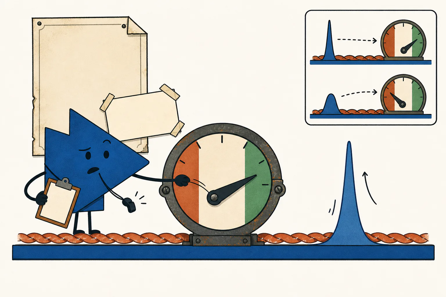
Why does SGD incur different fresh nuisance error at the same signal response? Inspect the actual example weights from the opening 100-point run. In the opening three-pass view, the loss plot above ends at update 300, so start with Inspect the first pass; the later updates show the corrections made on reuse.
Write u = Σi αixi. Each stem below is one αᵢ, that point’s weight. Each point carries signal together with its own nuisance. In the first pass, at the “Useful first pass” rate, stylized weights decay geometrically: early points receive more because more signal error remains. On reuse, corrections can reverse their signs. With iid inputs, signal values and nuisance overlaps also affect each coefficient.
100 examples; orthogonal nuisance; exact labels
Each stem is a calibration record’s actual coefficient. Its contribution to the recovered physical signal is αᵢ times the alignment between that record and the sensor-response direction. The same current predictor supplies all four readouts.
Each stem is its point’s coefficient αᵢ. With iid data, the signal contribution also depends on its label yᵢ: a negative coefficient can carry useful signal when its label is negative. Inspect a stem to see both. The scores below use this draw’s actual nuisance geometry.
This slider chooses the SGD update. The stems above are ordered by example, not by update.
Equal-weight comparison: the same signal, spread equally across all 100 points, including any not yet used by SGD. This is a comparison predictor, not another SGD step.
Let s = Σ αi and V = Σ αi² − s²/n ≥ 0. Equalizing all n weights to s/n preserves the signal. The comparison is a counterfactual predictor, not an SGD update.
Test error = (γs − 1)² + (d−1)(s²/n + V)
Training error = ((γ + (d−1)/n)s − 1)² + ((d−1)²/n)V
The extra cost of unequal weights is (d−1)V on test and (d−1)²V/n on training. Training amplifies that extra cost by (d−1)/n = 500.
Each row of X is one calibration record. As elsewhere on this page, rows are examples. Write G = XXᵀ, b = Xa and u = Xᵀα. Then:
r = bᵀα; test error = (r − 1)² + σ²αᵀGα.
Training error = ‖Gα − y‖² / ‖y‖².
Write each input as xᵢ = (√γ yᵢ, zᵢ) and let Wᵢⱼ = ⟨zᵢ, zⱼ⟩ be its nuisance Gram matrix. For the displayed coefficients, put s = Σ αᵢyᵢ.
Test error = (γs − 1)² + αᵀWα
Training error / predicting zero = Σᵢ ((γs − 1)yᵢ + (Wα)ᵢ)² / Σᵢ yᵢ²
Equal coefficients need not preserve the signal here, and nuisance cross terms matter. The equal-weight comparison and participation formula apply to the stylized model; iid mode reports the actual test and training scores instead.
The default weight scale is ±2η: in the stylized model, the very first update reaches halfway to the top. In iid mode that first coefficient is ηy₁, so its height depends on the sampled label. “Show full weight range” instead uses one common scale for the entire three-pass trajectory.
In the stylized model, equal positive weights give neff = n. Concentrating the same signal into fewer points costs more nuisance. That familiar effective-sample-size idea explains part of the price SGD pays compared with the best-in-span predictor: the weighting of these 100 points with the lowest fresh-test error.
On the stylized first pass, the exact weights in arrival order are αi = η(1 − ηγ)i−1. Making the signal bias very small requires enough cumulative progress, but it also makes this profile less uniform. For a long, slowly decaying geometric window, neff ≈ 2/(ηγ) − 1. Driving the bias down to a small target therefore introduces a logarithmic participation penalty. The finite profile above is exact; this window estimate is asymptotic.
Oja’s streaming principal component analysis (PCA) experiment has the complementary memory pattern. In its orthogonal preview, the growing direction and successive normalizations make recent contributions relatively stronger. The shared idea is concentration of sample weights, not identical supervised and unsupervised dynamics.
A and B are families of problems, one per size M. At each size they share their target, its two amplified directions (target modes, one weaker than the other), the training sample count and unamplified nuisance tail.
Only the amplified directions the target ignores—the unused modes—are stronger in B.
A’s one-pass test error keeps falling as the family grows. In B, the stronger unused modes obstruct recovery of the weaker target mode. As the families grow, span-restricted negative ridge drives test error to zero in both.
The two Gram systems above show the difference. Negative ridge and one-pass SGD can both cancel most of the nuisance diagonal in the multispike example, but ridge chooses all the example coefficients jointly, while SGD commits each coefficient from the residual the moment its point arrives. While the weak target mode is still being learned, those residuals stay large and feed variance into the strong unused modes. The Function Space matched-pair experiment shows this conflict while keeping the target modes fixed.
Equal-band paper reference: after one pass of 256 fresh examples, expected error is about 0.066 in A and 0.22 in B, each at its own rate. Explore the matched pair and why one rate faces this conflict.
Drag the cursor or a point sideways to choose a family size. A uses its prescribed rate; B uses the best of 80 preset rates for that size. Each rate stays fixed during its pass.
| Family | Expected fresh-test error | Expected error in the two target modes |
|---|---|---|
| A | ||
| B |
These are Gaussian expected risks, averaged over training draws, from the same one-pass recurrence used in Function Space. The finite sweep illustrates the comparison; the asymptotic theorem establishes the nonvanishing-risk obstruction along B for every predetermined positive constant rate.
Freeze a trained predictor and change only its test law to distinguish missed signal from error magnified by higher-variance test inputs.
Why choose coefficients jointly? Imagine two examples whose useful components agree and whose unwanted components oppose. Equal coefficients cancel the unwanted response. Chronological SGD generally gives them different coefficients. The two-example calculation makes this exact; the iid experiment below tests richer geometry.
Family A · slightly distinct strengths · M = 16, n = 256
In the opening A example, one pass learns both target modes while fitting its own examples badly. B strengthens unused modes, holding the random draws, labels, order, rate and nuisance tail fixed. This 256-example experiment is separate from the growth controls above.
The checked default comparison is available below. Interactive controls activate when the experiment is ready.
On the predetermined iid draw with slightly distinct strengths, the original two-mode task and 256 examples, A’s completed SGD fresh-test error is 0.062591, versus 0.081957 for illustrative negative ridge. A’s exact expected SGD error is 0.066187. Its training error is about 23,269 times that of predicting zero: useful learning coexists with severe misfit.
Changing only the fifteen unused strengths to B, at the same numeric rate, gives selected-draw SGD error 0.683380 and ridge error 0.087001. Adjusting B’s SGD rate gives 0.227977. B’s training error relative to predicting zero is about 121,202 at A’s rate and 19,507 at B’s adjusted rate. These are selected-draw outcomes, not universal rate bounds. The explanation drawers and exact two-example calculation remain available below.
Ridge shift accepted: the shifted Gram matrix is positive definite.
Both completed predictors use all 256 examples. Target held fixed across training draws.
Across 64 independent training sets: The matching 64-draw summary loads separately from this selected experiment.
Exact Gaussian mean for SGD: 0.066187. It averages SGD’s fresh-test error over new training sets; the selected draw’s score and the cohort median are shown separately.
| Learner | Median | 10th–90th percentiles | Below predicting zero |
|---|
Successful A comes first. Compare B at the same rate, then adjust the rate for B to see the compromise.
With the original task, try three comparisons: A succeeds; B at the same rate adds fluctuations; reducing B’s rate trades less fluctuation for slower weak-mode recovery.
Exact Gaussian expectations for this fixed target on new training sets.
Completed-pass mean weak response: 0.531; target coefficient: 0.707 (50% of label variance).
Completed-pass total expected error: squared bias 0.0310 + variance 0.0352 = 0.0662.
The plots share rulers across the A/B comparisons.
Responses here are signed coefficients of standardized modes. Divide by a mode’s nonzero target coefficient to obtain its gain, as in Function Space: gain 1 means full recovery. One learning rate need not give every mode the same gain.
Completed pass. Scrubbing changes the prefix readings; the headline and across-draw summary continue to describe the completed predictors.
Named presets refer to this spectrum and the original task. A’s rate is prescribed; B’s minimizes exact expected error on a declared grid. Editing the target, family, spectrum or draw keeps the numeric rate. Ridge has its own setting.
Predict before trying: if we reorder these same examples, which completed predictor should change?
Shuffling changes SGD’s chronology, not the dataset. Ridge’s completed predictor is unchanged by a permutation. “New iid draw” generates independent inputs, retaining the task and tuning.
Here d₀ is the number of unamplified nuisance coordinates. The illustrative shift is nλ = (5/2)√(nd₀) − d₀. Both named ridge recipes check their allowed spectral branch and fall back to predicting zero on rejection. A custom shift has no attached expected-risk theorem.
A first pass keeps the point’s own self-comparison out of its update. Earlier updates still affect its prediction through shared feature directions. Start with the first interaction, then compare a later update.
The predictor is zero before the first update. All modal responses and stored nuisance are zero; no arriving example has supplied a coefficient yet.
Before this update: contributions to this example. Residual = label − prediction.
| Group | Desired | Predicted | Residual part desired − predicted |
|---|---|---|---|
| Weak mode | sᵢ,weak times the desired and predicted responses | ||
| Original strong mode | sᵢ,1 times the desired and predicted responses | ||
| Unused modes | Sum over the same fifteen feature directions | ||
| Nuisance | 0 | Earlier examples’ nuisance overlaps | |
Before the selected update, compare each group’s signed contribution to this example with its fresh-error cost. These are different measurements.
These bars show contributions to this example’s prediction. The history measures errors across fresh inputs. A smaller unwanted predictor can still contribute more strongly on this particular example.
The nuisance increment can have either sign: a new contribution can partly cancel the previous nuisance predictor.
Follow the selected row’s earlier contributions, diagonal term, and later contributions into the parallel equations.
These are the same parallel equations, now evaluated on the selected multispike example. SGD fixes a historical coefficient on arrival. Ridge chooses its coefficients jointly using all 256 examples.
Both use the same Gram matrix. The comparison changes both chronology and the diagonal prescription: SGD retains earlier interactions with diagonal η⁻¹; ridge retains both triangles and shifts the original diagonal. Symmetry lets the upper entries be recovered from the lower ones: the contrast is in the equations used, not information missing from the dataset.
No update is selected before the first arrival. The general coefficient systems and nuisance-offset comparison still apply.
| Term | One-pass SGD | Joint ridge |
|---|---|---|
| Matrix diagonal, before multiplying | η⁻¹ | Kᵢᵢ + nλ |
| Earlier-index contribution | Σₕ<ᵢ Kᵢₕαˢₕ | Σₕ<ᵢ Kᵢₕαᴿₕ |
| Diagonal contribution | η⁻¹αˢᵢ | (Kᵢᵢ + nλ)αᴿᵢ |
| Later-index contribution | 0 | Σₕ>ᵢ Kᵢₕαᴿₕ |
| Sum of the three weighted contributions | yᵢ | yᵢ |
The bare matrix diagonal is not an additional summand. Ridge’s earlier-index terms use ridge’s own coefficients. A rejected ridge solve shows the fallback to predicting zero instead of claiming a solved row balance.
Predict before trying: if we reorder these same examples, which completed predictor should change?
Follow the completed example coefficients and the scores here. Reordering changes which predictions SGD has already made; ridge solves the same joint equations with their rows and columns relabeled.
Orthogonal nuisance disappears from first-pass coefficient feedback but returns when the predictor meets its training examples. Write d₀ for the number of unamplified nuisance coordinates. To isolate this geometry, set W = d₀I and hold the rate and signal inputs fixed. Then K = d₀I + SΓSᵀ, but the strictly earlier entries contain only signal interactions.
The coefficients here do not depend on d₀ at a fixed rate; the nuisance penalty and retrospective training error do. Signal error can partly cancel the returning nuisance. The regular-grid Fourier lab realizes this orthogonality exactly: each point’s nuisance lobe vanishes at the other training points. The live iid experiment instead retains its actual nuisance overlaps.
Frozen matched penalty λη = ; active iid penalty λ = .
The two penalties can nearly coincide while the coefficient equations remain different. After matching the frozen nuisance offset, ridge retains the signal self-term and both earlier and later couplings; SGD retains strictly earlier interactions. Compare the operative diagonals and weighted row contributions above. This frozen comparison uses the analyst’s d₀, not a third ridge setting. The earlier twelve-example animation’s positive shift and the scalar signal-response match make different comparisons.
A negative matched penalty guarantees that a nonzero arriving residual crosses the label in this frozen geometry, since Kᵢᵢ ≥ d₀. Crossing needs ηKᵢᵢ > 1; increasing the point’s squared loss needs ηKᵢᵢ > 2. A zero residual remains zero. The whole-batch training-error curve must be checked separately.
Keep the inputs, example order and both learner rules fixed. First move some of the original strong task into other modes while keeping half the label variance in the weak mode. Then change the weak share itself.
Completed fresh-test errors: SGD 0.062591 · ridge 0.081957.
The all-mode preset assigns 50% to the weak mode, 40% to the original strong mode and 10% spread equally over all fifteen others. Slightly distinct strengths make all seventeen feature eigenmodes identifiable.
Nuisance is the unamplified feature tail. It is distinct from amplified modes that the current target leaves unused.
A mode is unused by this target when its target coefficient is zero; the learned predictor can still respond in that direction.
When any of the fifteen modes participates, its fixed group is called “Other modes.” A/B still changes those fifteen feature strengths, while keeping the standardized target and paired labels fixed; some changed directions now help define the task.
These are signed relative coefficients: after normalization, each coefficient’s square is its share of label variance. Changing one changes the others’ normalized shares. At least one mode must contribute. Negative weights reverse the desired response; zero means that feature direction is unused by this target.
Return to the response and error histories for this task.
Target edits change the labels and desired responses without retuning either learner. In the equal-band reference only, redistributing a fixed share within an equal-strength eigenspace preserves exact mean risk; an individual draw can still change.
Here is the two-example cancellation in full. This constructed example and its all-rate bound are distinct from the iid evidence.
| Rule | Weak response | Unwanted strong response | Fresh-test error |
|---|---|---|---|
| Best positive constant-rate SGD | 0.449762 | −0.378414 | 0.456520 |
| Best nonnegative ridge (λ = 0) | 0.166667 | 0 | 0.695833 |
| Negative ridge (λ = −500) | 1 | 0 | 0.050000 |
| Test-optimal ridge here (λ = −495) | 0.952381 | 0 | 0.047619 |
Both labels are 1. Nonnegative ridge coordinates the cancellation but leaves too little weak response; the negative shift corrects the shrinkage.
SGD’s second coefficient responds to the first update’s wrong-sign strong prediction. The best positive constant rate is approximately 0.001775795, but every positive constant rate has error at least 4/9. Write ξ = 100η:
The squared distance from the desired response (1,0) to this half-space is 4/9; nuisance adds a nonnegative cost. This bound and the numerical minimum answer different questions. The best-span value 1/21 happens to be achieved by ridge here; ridge and best in span are different notions in general.
In a complete orthogonal construction, take one constant weak column and n − 1 orthogonal unused columns, each of squared length n and common strong strength. Then the unused directions detect differences between example coefficients:
This extends the participation lesson: uneven participation has a cost beyond nuisance. The repeated strengths and complete orthogonality are intentional here. Random columns instead require the signed projections shown in the live inspector; the toy’s flat ridge coefficients and exact cancellation do not transfer automatically.
Cancellation means a small signed projection onto a feature pattern. It does not require equal coefficients on random examples.
Completed pass. The default inspection is the original strong mode; compare its desired response with both learners’ responses and squared errors. The third history trace keeps its selected other mode.
For the selected output j, the own-mode term includes its desired response; each other term is the response induced by that label mode. Add these signed terms before squaring.
| Label mode | Signed target weight βₖ | SGD error contribution | Ridge error contribution |
|---|
The selected input mode is highlighted. Opposite signs can cancel across requested modes even when every mode has positive label-variance share.
A unit input probe shows how the fixed learner responds to one label pattern. Its actual contribution is multiplied by that mode’s signed target weight. Selecting a mode highlights it without changing the task.
For either learner, the inverse coefficient system maps the labels to example coefficients:
Choose the corresponding inverse in the expressions below. The triangular mask and joint ridge solve therefore produce two different response maps from the same label patterns.
In the response tables, input label modes are columns and output modes are rows. The ideal is the identity. Each unit response remains fixed when the target changes; its actual contribution scales with β. Squared own- and cross-mode pieces are not additive, because their signed contributions can cancel.
One rate constructs different mean gains in different modes. This mean omits the fluctuations measured by the error history. The response maps omit fresh nuisance error, which remains included in the completed fresh-error scores above.
Carry the selected output mode into this completed-pass comparison. What signed change turns its SGD error into its ridge error? A joint correction can improve some modes while worsening others. Here Aᴿ = K + nλI is the ridge system, and C maps example coefficients into the population-weighted responses defined below.
The correction concerns the completed predictors, even when the history is scrubbed to an earlier example.
| Quantity | Value |
|---|---|
| Selected example: equation residual | |
| Later-index contribution | −UαS |
| Changed diagonal and shift | [η⁻¹I − D − nλI]αS |
| Combined residual | z |
The selected mode changes by γⱼ⟨s:ⱼ, δα⟩. The two sources of the residual can reinforce or cancel; neither is guaranteed to help independently. This exact retrospective identity explains the predictor difference. The update history and recurrence explain how SGD accumulated its error.
The cross term matters, and the total risk change can have either sign. This is not an animation of a third learning algorithm. The correction is available only when the selected ridge solve passes its spectral check.
A direction with a large error gain matters when the target aligns with it. The relevant map measures prediction error in the population metric, including nuisance. The triangular system’s eigenvalues alone—all η⁻¹—cannot reveal this task-dependent error.
Start with the same two inverses: 𝒯ₛ = (η⁻¹I + K<)⁻¹ and 𝒯ᵣ = (K + nλI)⁻¹. Target weights make labels; the chosen inverse makes example coefficients; their population-weighted error is what the singular gains measure.
Research Context distinguishes averaging predictors from averaging their squared errors; the same covariance-weighted metric tells us which errors are expensive here.
Each learner defines its own singular directions. To compare a direction fairly, keep one selected unit target fixed and evaluate it with both learners below.
| Learner | Weak | Original strong | Other modes | Nuisance | Total |
|---|
| Learner | Fresh-test error | Error-gain reconstruction |
|---|---|---|
| One-pass SGD | ‖ESβ‖² | |
| Negative ridge | ‖ERβ‖² | |
Changing the target moves its alignments without changing either learner’s error map. A rate change changes SGD’s map; a ridge-setting change changes ridge’s map.
Inspecting a direction leaves the task unchanged. The button below explicitly applies its signed weights to both learners.
A target chosen from this draw is marked as dataset-selected and stays frozen on redraw. Its same-draw score is descriptive; expected-risk results for a predetermined target concern independent new datasets. Nearly tied directions have a stable subspace interpretation, even if a particular basis inside that subspace changes.
The selected-direction comparison scores one common unit target. Actual group errors for the current task come from the full signed sum Eβ; combining per-direction group costs with squared alignments alone would omit cross terms. This target’s alignment weights describe its own error; the full singular spectrum describes the operator. What does the learning rule add beyond norm and training error? Context compares those summaries on a separate finite multispike draw; its one-spike tuned-SGD guarantee has different scope.
Each mode responds to common error and adds to the error driving later updates. Research Context follows this exchange between one signal and nuisance; here several amplified modes also contribute.
To isolate one injection, suppose only the weak task remains wrong and the nuisance predictor is zero. A fresh example then writes into an unused mode j:
Here εⱼ = βⱼ − aⱼ is modal shortfall; rᵢ is the scalar residual on an arriving example. Opposite signed predictions can cancel in the mean while their squared prediction errors remain.
These exact Gaussian recurrences evolve expected squared error in all seventeen modes and the nuisance tail. They produce the dashed total-error history. They do not assert monotone growth on each draw.
For the original task, A and B at the same numeric rate have identical mean weak and original-strong responses. The extra expected error comes from variance. When changed feature directions participate in a dense task, that comparison no longer holds.
Let V be total expected error in the fifteen other modes, and X the error in the two original target modes plus nuisance. For a moment, hold the external forcing X constant:
This equilibrium requires 0 < ηγⱼ < 1 for all fifteen modes and G < 1. G includes injection and persistence over time; it is not a one-step reinjection fraction. In the default distinct spectrum, G is about 0.042 in A at A’s rate, 0.732 in B at that same rate, and 0.428 after adjusting B’s rate.
The live X changes. Its earlier values continue to affect the current error, so this equilibrium is an explanation, not a replacement curve. In default B at A’s rate the collective block’s slow decay takes about 23 updates; this is different from the eight-update gap between its total-risk and other-mode peaks.
These are classical Gaussian least-mean-squares (LMS) second-moment dynamics; see Sayed, Adaptive Filters, Chapters 22–23, as discussed in the Multispike preprint. The familiar misadjustment calculation reappears when we freeze the error driving the other modes. Our update convention is w⁺ = w + ηrx; a convention using 2μrx needs conversion.
In a stable full Gaussian LMS system with independent label-noise variance σ², stationary excess prediction error divided by σ² is Gfull/(1 − Gfull). Here the labels are noiseless, the forcing evolves, and the fifteen-mode G is only a subsystem. Its roughly 2.736 frozen amplification in default B is not a whole-system steady-state misadjustment.
| Question | What the calculation says |
|---|---|
| Mean signal recovery | The mean response contracts with factors 1 − ηγⱼ; it omits variance. |
| Fifteen-mode frozen forcing | G < 1 supports the stated subsystem equilibrium. |
| Indefinite fresh-stream mean-square stability | The full system includes nuisance. Gfull is about 177.5 in default A and 178.2 in B, outside the stable domain despite A’s useful finite pass. |
| Useful finite-pass learning | There must be enough progress in the weak mode before accumulated signal and fresh nuisance errors become too large. |
| Repeatedly optimize training loss | A different objective on reused data; see One rate, five different questions. |
The growing distinct-spectrum families separate an algorithmic obstruction from an information limit. A’s prescribed pass succeeds in expected risk, and conservative spectral-margin negative ridge succeeds in both families, uniformly over predetermined unit targets. Their training errors, including errors relative to predicting zero, diverge in probability. Useful learning can require misfitting even when every feature mode helps define the task.
For B, no predetermined positive constant rate makes expected error vanish along the family when the weak label share w stays positive:
The dense preset keeps w = 1/2. Removing the weak task removes this positive floor. At M = 16 with the 5% spread in unused-mode strengths (δ = 0.05), this lower bound is about 0.0104. The exact recurrence gives expected error about 0.22 for B at B’s rate and 0.77 for B at A’s rate, as shown in the expected-error history above. The bound establishes an obstruction across all positive constant rates; it is not a tight prediction of these finite errors. The result does not assert failure on most draws, for variable-rate schedules, or for every data-dependent tuning rule.
Enough weak-mode progress requires θ to grow, while the sufficient window controls θq and θ²/Rwk. A permits these together; B’s signal trace exposes the compromise. The finite-row ledger, stochastic recurrence and error-map SVD explain chronology, collective cost and target alignment, respectively.
The theorem uses the Conservative spectral margin ridge recipe, not the illustrative curve. A passed matrix check does not certify low realized test error. Dense A/B comparisons retain the standardized target and paired labels while changing some participating strengths; physical oracle coefficients βⱼ/√γⱼ change, and each family is scored under its own law. See the preprint’s distinct-dense corollary and proof for the exact scope.
A hump follows error across successive predictors; misfitting compares training and fresh errors for one predictor. Compare loss on arriving examples with the current predictor’s loss on the stored batch. Measuring before an update does not make a reused example fresh.
Recall the opening loss explanation; its arriving-loss controls are in “Model, draw, order and detailed scores.”
The cursor marks the same transition in both views. The whole-batch score is measured after the update.
The fresh-arrival identity assumes a target, rate and order chosen independently of that draw. With replacement from retained data, an independent uniform next index instead measures empirical loss on that dataset; reshuffling only the remaining examples does not generally give that identity. A target chosen by inspecting this draw keeps its realized log, but its fresh-data interpretation applies after an independent redraw with that target frozen.
All three moving averages use the same debiased weights, with smoothing 0.9. They summarize preceding predictors, so they lag behind changes.
| Connection | What that curve measures | What carries over here |
|---|---|---|
| Nakkiran et al., Deep Double Descent (§6, Figs. 9–10) | Test error over repeated epochs on retained data: descent, ascent, descent. | Nonmonotone generalization over training time. Here the expected risk can rise immediately then fall during one fresh pass; neither the full shape nor an interpolation explanation has been established. |
| Lewkowycz et al., The Catapult Mechanism (§2.1, Fig. 2) | Loss on the same retained example, repeatedly used for training. | In that experiment, training loss rises and then falls as curvature changes. Here the arriving-loss log and retrospective training loss ask different questions, and this fixed quadratic has no such curvature change. |
| Heckel and Yilmaz, Early Stopping in Deep Networks (§2, Fig. 2) | Differently timed spectral bias–variance tradeoffs with fixed noisy data. | Spectral timescales offer a useful connection. Here the labels are noiseless, and fresh updates create stochastic excitation that can later relax. |
Adaptive-filtering readers will recognize an LMS learning curve; the recurrence explanation connects its transient behavior to classical second-moment dynamics.
This experiment uses seventeen amplified Gaussian feature modes plus an unamplified nuisance tail, 256 iid training examples and exact labels. In the original task only the weak and original strong modes have nonzero label share. Family A and B share the same standardized inputs and nuisance draw.
Seed: 20261002. The website’s JavaScript draws and the independent Python manuscript archive use different sampling protocols: equal seed numbers do not mean equal datasets. The cohort retains all its outcomes. Target-selected cohort rescoring is descriptive; it does not establish performance of that selection procedure on independent targets.
η sets the update size. βⱼ is mode j’s signed target weight. aⱼ is the predictor’s signed response in mode j. γⱼ is mode j’s population feature strength. sᵢⱼ is example i’s standardized entry in mode j. rᵢ is the label minus its before-update prediction. νᵢ is the arriving prediction from earlier nuisance contributions. λ is the ridge penalty; nλ shifts the Gram diagonal. E maps target weights to population-weighted prediction error. κℓ is the error gain for a unit target direction. vℓ is a unit direction in target space.
Displayed settings are rounded for readability; calculations and saved settings retain full precision.
Default: A; distinct strengths; original target; original order; A’s numeric rate; illustrative ridge shift; completed pass, paused.
Compare this experiment in Function Space.
In the single-spike example, a well-chosen large-rate pass restores signal while storing nuisance. With several spikes, stronger unused directions can obstruct SGD even when negative ridge succeeds. Reuse adds a separate problem: stored nuisance feeds back into later updates.
Function Space shows what these weights draw. The Research Context page explains why fresh-stream and fixed-dataset traditions naturally watch different losses.
A fresh stream is not safe forever at a fixed aggressive rate either. For fresh iid Gaussian examples at the opening parameters and rate 2 × 10⁻⁴, expected test error bottoms out near update 149 and is worse than predicting zero again by update 1,852 (Research Context: One rate, five different questions).